Chapter 5 Linear Models
##
## Attaching package: 'dplyr'
## The following objects are masked from 'package:stats':
##
## filter, lag## The following objects are masked from 'package:base':
##
## intersect, setdiff, setequal, union## Loading required package: StanHeaders## rstan (Version 2.16.2, packaged: 2017-07-03 09:24:58 UTC, GitRev: 2e1f913d3ca3)## For execution on a local, multicore CPU with excess RAM we recommend calling
## rstan_options(auto_write = TRUE)
## options(mc.cores = parallel::detectCores())## Loading required package: parallel## Loading required package: methods## rethinking (Version 1.59)##
## Attaching package: 'rethinking'## The following object is masked from 'package:purrr':
##
## maploading the tadpole data
data("reedfrogs", package = "rethinking")

d <- reedfrogs
glimpse(d)
## Observations: 48
## Variables: 5
## $ density <int> 10, 10, 10, 10, 10, 10, 10, 10, 10, 10, 10, 10, 10, 1...
## $ pred <fctr> no, no, no, no, no, no, no, no, pred, pred, pred, pr...
## $ size <fctr> big, big, big, big, small, small, small, small, big,...
## $ surv <int> 9, 10, 7, 10, 9, 9, 10, 9, 4, 9, 7, 6, 7, 5, 9, 9, 24...
## $ propsurv <dbl> 0.90, 1.00, 0.70, 1.00, 0.90, 0.90, 1.00, 0.90, 0.40,...Here is a model which fits a separate intercept for each tank in these frogs
# specify model
## one intercept per tank
one_per_tank <- alist(
  surv     ~ dbinom(density, p),
  logit(p) ~ a_tank[tank],
  a_tank[tank] ~ dnorm(0, 5) ## I guess that magically knows that it needs to make 48?
)

m12.1 <- d %>%
  mutate(tank = seq_along(density)) %>%
  rethinking::map2stan(one_per_tank, data = .)
## In file included from fileca8524dd3bf.cpp:8:
## In file included from /Library/Frameworks/R.framework/Versions/3.4/Resources/library/StanHeaders/include/src/stan/model/model_header.hpp:4:
## In file included from /Library/Frameworks/R.framework/Versions/3.4/Resources/library/StanHeaders/include/stan/math.hpp:4:
## In file included from /Library/Frameworks/R.framework/Versions/3.4/Resources/library/StanHeaders/include/stan/math/rev/mat.hpp:4:
## In file included from /Library/Frameworks/R.framework/Versions/3.4/Resources/library/StanHeaders/include/stan/math/rev/core.hpp:12:
## In file included from /Library/Frameworks/R.framework/Versions/3.4/Resources/library/StanHeaders/include/stan/math/rev/core/gevv_vvv_vari.hpp:5:
## In file included from /Library/Frameworks/R.framework/Versions/3.4/Resources/library/StanHeaders/include/stan/math/rev/core/var.hpp:7:
## In file included from /Library/Frameworks/R.framework/Versions/3.4/Resources/library/BH/include/boost/math/tools/config.hpp:13:
## In file included from /Library/Frameworks/R.framework/Versions/3.4/Resources/library/BH/include/boost/config.hpp:39:
## /Library/Frameworks/R.framework/Versions/3.4/Resources/library/BH/include/boost/config/compiler/clang.hpp:200:11: warning: 'BOOST_NO_CXX11_RVALUE_REFERENCES' macro redefined [-Wmacro-redefined]
## # define BOOST_NO_CXX11_RVALUE_REFERENCES
## ^
## <command line>:6:9: note: previous definition is here
## #define BOOST_NO_CXX11_RVALUE_REFERENCES 1
## ^
## 1 warning generated.
##
## SAMPLING FOR MODEL 'surv ~ dbinom(density, p)' NOW (CHAIN 1).
##
## Gradient evaluation took 1.5e-05 seconds
## 1000 transitions using 10 leapfrog steps per transition would take 0.15 seconds.
## Adjust your expectations accordingly!
##
##
## Iteration: 1 / 2000 [ 0%] (Warmup)
## Iteration: 200 / 2000 [ 10%] (Warmup)
## Iteration: 400 / 2000 [ 20%] (Warmup)
## Iteration: 600 / 2000 [ 30%] (Warmup)
## Iteration: 800 / 2000 [ 40%] (Warmup)
## Iteration: 1000 / 2000 [ 50%] (Warmup)
## Iteration: 1001 / 2000 [ 50%] (Sampling)
## Iteration: 1200 / 2000 [ 60%] (Sampling)
## Iteration: 1400 / 2000 [ 70%] (Sampling)
## Iteration: 1600 / 2000 [ 80%] (Sampling)
## Iteration: 1800 / 2000 [ 90%] (Sampling)
## Iteration: 2000 / 2000 [100%] (Sampling)
##
## Elapsed Time: 0.207582 seconds (Warm-up)
## 0.178872 seconds (Sampling)
## 0.386454 seconds (Total)
##
##
## SAMPLING FOR MODEL 'surv ~ dbinom(density, p)' NOW (CHAIN 1).
##
## Gradient evaluation took 1.2e-05 seconds
## 1000 transitions using 10 leapfrog steps per transition would take 0.12 seconds.
## Adjust your expectations accordingly!
##
##
## WARNING: No variance estimation is
## performed for num_warmup < 20
##
## Iteration: 1 / 1 [100%] (Sampling)
##
## Elapsed Time: 0 seconds (Warm-up)
## 8.9e-05 seconds (Sampling)
## 8.9e-05 seconds (Total)## Warning: There were 1 divergent transitions after warmup. Increasing adapt_delta above 0.8 may help. See
## http://mc-stan.org/misc/warnings.html#divergent-transitions-after-warmup## Warning: Examine the pairs() plot to diagnose sampling problems## Computing WAIC## Constructing posterior predictions## [ 100 / 1000 ]
[ 200 / 1000 ]
[ 300 / 1000 ]
[ 400 / 1000 ]
[ 500 / 1000 ]
[ 600 / 1000 ]
[ 700 / 1000 ]
[ 800 / 1000 ]
[ 900 / 1000 ]
[ 1000 / 1000 ]## Aggregated binomial counts detected. Splitting to 0/1 outcome for WAIC calculation.rethinking::precis(m12.1, depth = 2)## Mean StdDev lower 0.89 upper 0.89 n_eff Rhat
## a_tank[1] 2.51 1.21 0.64 4.27 1000 1
## a_tank[2] 5.77 2.78 2.01 10.32 1000 1
## a_tank[3] 0.91 0.71 -0.26 2.03 1000 1
## a_tank[4] 5.71 2.73 1.71 9.54 1000 1
## a_tank[5] 2.56 1.22 0.73 4.29 1000 1
## a_tank[6] 2.54 1.21 0.81 4.27 1000 1
## a_tank[7] 5.62 2.68 1.81 9.76 1000 1
## a_tank[8] 2.45 1.11 0.62 3.93 1000 1
## a_tank[9] -0.43 0.68 -1.45 0.61 1000 1
## a_tank[10] 2.47 1.06 0.89 4.15 1000 1
## a_tank[11] 0.93 0.73 -0.23 2.08 1000 1
## a_tank[12] 0.46 0.71 -0.63 1.66 1000 1
## a_tank[13] 0.91 0.69 -0.19 1.98 1000 1
## a_tank[14] -0.01 0.67 -1.01 1.02 1000 1
## a_tank[15] 2.49 1.13 0.67 4.14 1000 1
## a_tank[16] 2.54 1.18 0.84 4.34 1000 1
## a_tank[17] 3.54 1.13 1.72 5.10 1000 1
## a_tank[18] 2.64 0.82 1.36 3.82 1000 1
## a_tank[19] 2.13 0.67 1.07 3.15 1000 1
## a_tank[20] 6.34 2.51 2.63 9.84 1000 1
## a_tank[21] 2.61 0.76 1.32 3.63 1000 1
## a_tank[22] 2.60 0.76 1.53 3.86 1000 1
## a_tank[23] 2.64 0.83 1.41 3.78 1000 1
## a_tank[24] 1.73 0.57 0.87 2.63 1000 1
## a_tank[25] -1.19 0.47 -1.90 -0.37 1000 1
## a_tank[26] 0.09 0.43 -0.56 0.78 1000 1
## a_tank[27] -1.74 0.59 -2.64 -0.83 1000 1
## a_tank[28] -0.59 0.44 -1.24 0.17 1000 1
## a_tank[29] 0.09 0.37 -0.51 0.71 1000 1
## a_tank[30] 1.45 0.53 0.63 2.30 1000 1
## a_tank[31] -0.78 0.42 -1.53 -0.21 1000 1
## a_tank[32] -0.41 0.41 -1.07 0.23 1000 1
## a_tank[33] 3.81 1.07 2.21 5.34 1000 1
## a_tank[34] 3.02 0.81 1.74 4.15 1000 1
## a_tank[35] 2.93 0.74 1.77 4.02 1000 1
## a_tank[36] 2.13 0.57 1.31 3.08 1000 1
## a_tank[37] 2.15 0.57 1.25 2.98 1000 1
## a_tank[38] 6.74 2.61 2.77 10.34 1000 1
## a_tank[39] 2.97 0.75 1.74 3.94 1000 1
## a_tank[40] 2.48 0.61 1.53 3.41 1000 1
## a_tank[41] -2.11 0.56 -3.04 -1.28 1000 1
## a_tank[42] -0.67 0.34 -1.23 -0.14 1000 1
## a_tank[43] -0.52 0.34 -1.04 0.01 1000 1
## a_tank[44] -0.42 0.36 -0.99 0.16 1000 1
## a_tank[45] 0.55 0.35 0.00 1.13 1000 1
## a_tank[46] -0.67 0.35 -1.24 -0.13 1000 1
## a_tank[47] 2.13 0.54 1.23 2.92 1000 1
## a_tank[48] -0.06 0.35 -0.63 0.46 1000 1or for the probabilaties of survival in any given tank
alphas <- rethinking::precis(m12.1, depth = 2)
rethinking::logistic(alphas@output[1, "Mean"])## [1] 0.9245589d[1, c("density", "surv", "propsurv")]## density surv propsurv
## 1 10 9 0.9OK so that’s pretty close to just calculating it right from the data.
varying_inters <- alist(
surv ~ dbinom(density, p),
logit(p) <- a_tank[tank],
a_tank[tank] ~ dnorm(mu, sigma),
mu ~ dnorm(0, 1),
sigma ~ dcauchy(0, 1)
)
m12.2 <- d %>%
mutate(tank = seq_along(density)) %>%
rethinking::map2stan(
varying_inters,
data = .
)## In file included from fileca834742465.cpp:8:
## In file included from /Library/Frameworks/R.framework/Versions/3.4/Resources/library/StanHeaders/include/src/stan/model/model_header.hpp:4:
## In file included from /Library/Frameworks/R.framework/Versions/3.4/Resources/library/StanHeaders/include/stan/math.hpp:4:
## In file included from /Library/Frameworks/R.framework/Versions/3.4/Resources/library/StanHeaders/include/stan/math/rev/mat.hpp:4:
## In file included from /Library/Frameworks/R.framework/Versions/3.4/Resources/library/StanHeaders/include/stan/math/rev/core.hpp:12:
## In file included from /Library/Frameworks/R.framework/Versions/3.4/Resources/library/StanHeaders/include/stan/math/rev/core/gevv_vvv_vari.hpp:5:
## In file included from /Library/Frameworks/R.framework/Versions/3.4/Resources/library/StanHeaders/include/stan/math/rev/core/var.hpp:7:
## In file included from /Library/Frameworks/R.framework/Versions/3.4/Resources/library/BH/include/boost/math/tools/config.hpp:13:
## In file included from /Library/Frameworks/R.framework/Versions/3.4/Resources/library/BH/include/boost/config.hpp:39:
## /Library/Frameworks/R.framework/Versions/3.4/Resources/library/BH/include/boost/config/compiler/clang.hpp:200:11: warning: 'BOOST_NO_CXX11_RVALUE_REFERENCES' macro redefined [-Wmacro-redefined]
## # define BOOST_NO_CXX11_RVALUE_REFERENCES
## ^
## <command line>:6:9: note: previous definition is here
## #define BOOST_NO_CXX11_RVALUE_REFERENCES 1
## ^
## 1 warning generated.
##
## SAMPLING FOR MODEL 'surv ~ dbinom(density, p)' NOW (CHAIN 1).
##
## Gradient evaluation took 2e-05 seconds
## 1000 transitions using 10 leapfrog steps per transition would take 0.2 seconds.
## Adjust your expectations accordingly!
##
##
## Iteration: 1 / 2000 [ 0%] (Warmup)
## Iteration: 200 / 2000 [ 10%] (Warmup)
## Iteration: 400 / 2000 [ 20%] (Warmup)
## Iteration: 600 / 2000 [ 30%] (Warmup)
## Iteration: 800 / 2000 [ 40%] (Warmup)
## Iteration: 1000 / 2000 [ 50%] (Warmup)
## Iteration: 1001 / 2000 [ 50%] (Sampling)
## Iteration: 1200 / 2000 [ 60%] (Sampling)
## Iteration: 1400 / 2000 [ 70%] (Sampling)
## Iteration: 1600 / 2000 [ 80%] (Sampling)
## Iteration: 1800 / 2000 [ 90%] (Sampling)
## Iteration: 2000 / 2000 [100%] (Sampling)
##
## Elapsed Time: 0.186412 seconds (Warm-up)
## 0.296387 seconds (Sampling)
## 0.482799 seconds (Total)
##
##
## SAMPLING FOR MODEL 'surv ~ dbinom(density, p)' NOW (CHAIN 1).
##
## Gradient evaluation took 1.4e-05 seconds
## 1000 transitions using 10 leapfrog steps per transition would take 0.14 seconds.
## Adjust your expectations accordingly!
##
##
## WARNING: No variance estimation is
## performed for num_warmup < 20
##
## Iteration: 1 / 1 [100%] (Sampling)
##
## Elapsed Time: 0 seconds (Warm-up)
## 7.7e-05 seconds (Sampling)
## 7.7e-05 seconds (Total)## Warning: There were 1 divergent transitions after warmup. Increasing adapt_delta above 0.8 may help. See
## http://mc-stan.org/misc/warnings.html#divergent-transitions-after-warmup## Warning: Examine the pairs() plot to diagnose sampling problems## Computing WAIC## Constructing posterior predictions## [ 100 / 1000 ]
[ 200 / 1000 ]
[ 300 / 1000 ]
[ 400 / 1000 ]
[ 500 / 1000 ]
[ 600 / 1000 ]
[ 700 / 1000 ]
[ 800 / 1000 ]
[ 900 / 1000 ]
[ 1000 / 1000 ]## Aggregated binomial counts detected. Splitting to 0/1 outcome for WAIC calculation.Then we compare the models
rethinking::compare(m12.1, m12.2)## WAIC pWAIC dWAIC weight SE dSE
## m12.2 1009.9 37.8 0 1 37.9 NA
## m12.1 1022.0 48.8 12 0 42.8 6.515.0.1 comparing multiple-intercepts to partial pooling
The more conservative approach – using the partial pooling – results in more accurate estimates
samps <- list(m12.1 = m12.1,
m12.2 = m12.2) %>%
map(rethinking::extract.samples)
## median for each tank, on log scale
post_median <- samps %>%
map(~ apply(.x[["a_tank"]], MARGIN = 2, FUN = median)) %>%
map(rethinking::logistic)
## note that if you want the different values of the parameter `a_tank` you need
## to get the element of the list named that (the other parameters are in there too).
## first the figure from the book:
post_median %>%
as.data.frame %>%
bind_cols(d, .) %>%
mutate(tank = seq_along(density)) %>%
select(density, tank, propsurv, m12.1, m12.2) %>%
tidyr::gather(datatype, prop_survival, propsurv, m12.1, m12.2) %>%
ggplot(aes(x = tank, y = prop_survival, fill = datatype)) +
geom_point(pch = 21) +
facet_grid(~density, scales = "free_x") +
scale_fill_brewer()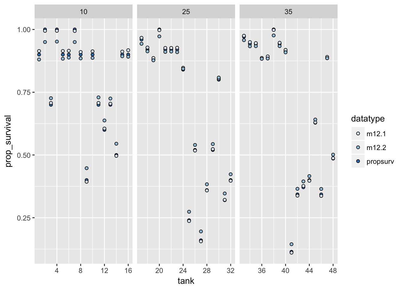
post_median %>%
as.data.frame %>%
bind_cols(d, .) %>%
mutate(tank = seq_along(density)) %>%
select(density, tank, propsurv, m12.1, m12.2) %>%
ggplot(aes(x = propsurv, y = m12.1)) +
geom_point(pch = 21, fill = "darkgrey") +
facet_grid(~density, scales = "free_x") +
coord_fixed(xlim = c(0, 1), ylim = c(0, 1)) +
geom_abline(slope = 1, intercept = 0) +
geom_point(aes(y = m12.2), pch = 21, fill = "red")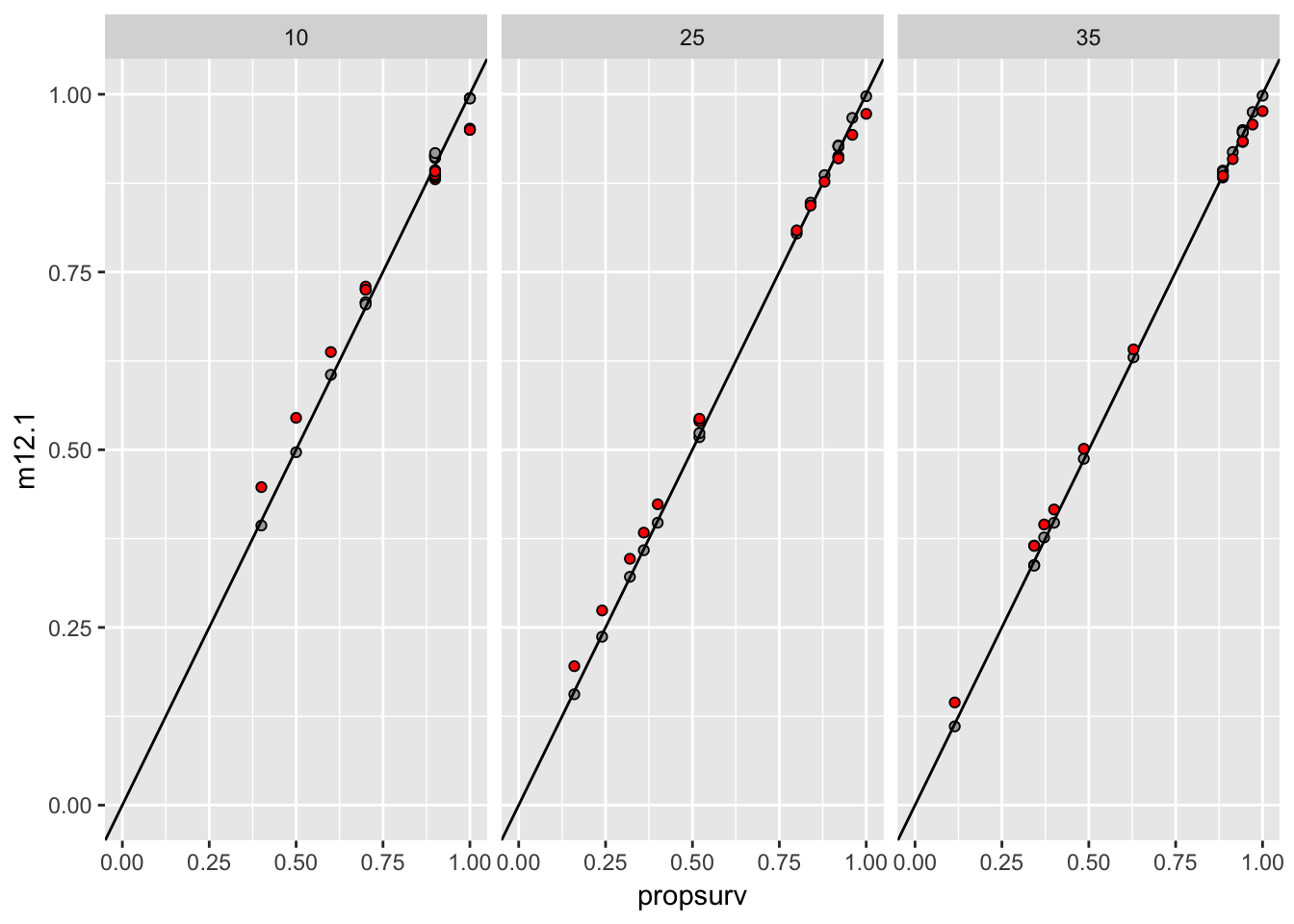
Figure 5.1: On the x-axis is the proportion suriving. On the Y, the proportion estimated in two different models. The grey points are from the no-pooling model, while the red ones are from the partial-pooling (hierarchical) model.
I guess the random effect “flattens” predictions slightly. Takes more exteme values less “seriously”. And the amount of flexibility is much higher for smaller samples.
5.0.1.1 the distribution of tanks
When we fit this model, we estimate that all tanks are coming from a distribution. What does that distribution look like? We have thousands of them, so we draw some samples to visualize:
post <- rethinking::extract.samples(m12.2)
plot(NULL, xlim = c(-3, 4), ylim = c(0, 0.35))
funs_norm <- post[c("mu", "sigma")] %>%
set_names(nm = c("mean", "sd")) %>%
transpose %>%
map(lift(partial), ...f = dnorm)
xs <- seq(-3, 4, length.out = 20)
normal_data <- funs_norm %>%
invoke_map(x = xs) %>%
map(cbind, xs) %>%
map(as.data.frame) %>%
bind_rows(.id = "samp_no")
normal_data %>%
ggplot(aes(x = xs, y = V1, group = samp_no)) +
geom_line(alpha = 0.04) +
theme_minimal()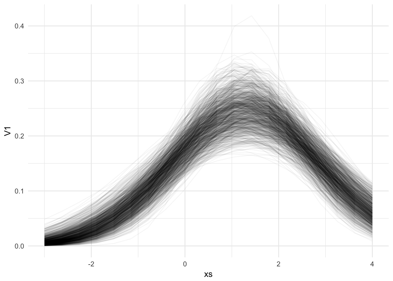
post[c("mu", "sigma")] %>%
set_names(nm = c("mean", "sd")) %>%
transpose %>%
map_df(~ data_frame(x = seq(-3, 4, length.out = 60),
y = dnorm(x, mean = .x$mean, sd = .x$sd))) %>%
bind_rows(.id = "sampling") %>%
ggplot(aes(x = x, y = y)) +
stat_bin_hex(aes(fill = ..density..), bins = 35)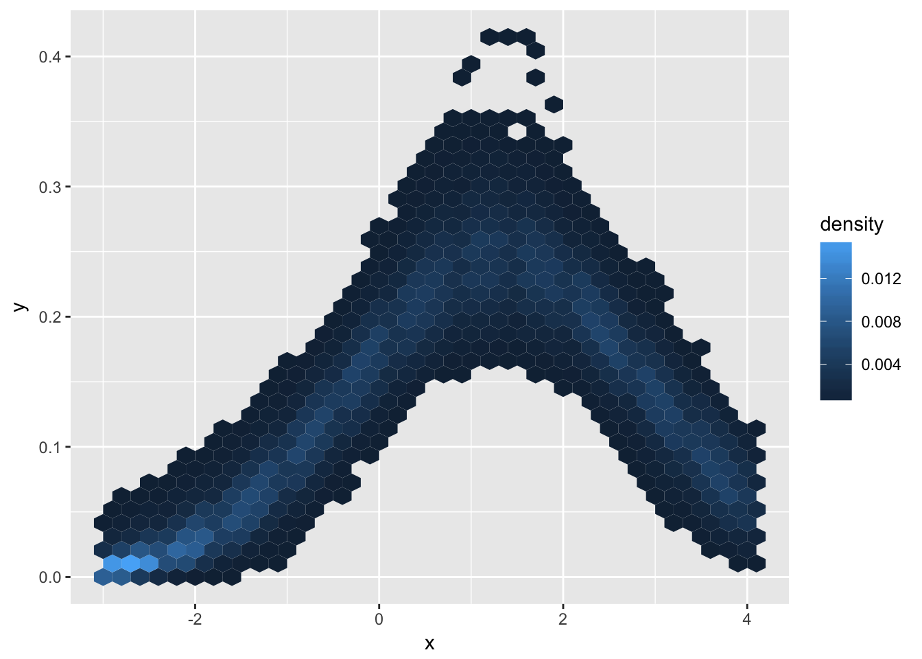
Or, we can visualize the uncertainty in survival across all tanks. To do that, we once again use the posterior samples. We use them to define a normal distribution and draw a single sample from it. Then, we convert it to survival probabilities with the inverse logistic function.
logistic_numbers <- post[c("mu", "sigma")] %>%
set_names(nm = c("mean", "sd")) %>%
transpose %>%
map(lift(rnorm), n = 1) %>%
# map_dbl(rethinking::logistic)
map_dbl(~ 1/(1 + exp(-.x)))
logistic_numbers %>% #data_frame(xs = .) %>% ggplot(aes(x = xs)) + geom_density()
rethinking::dens(.)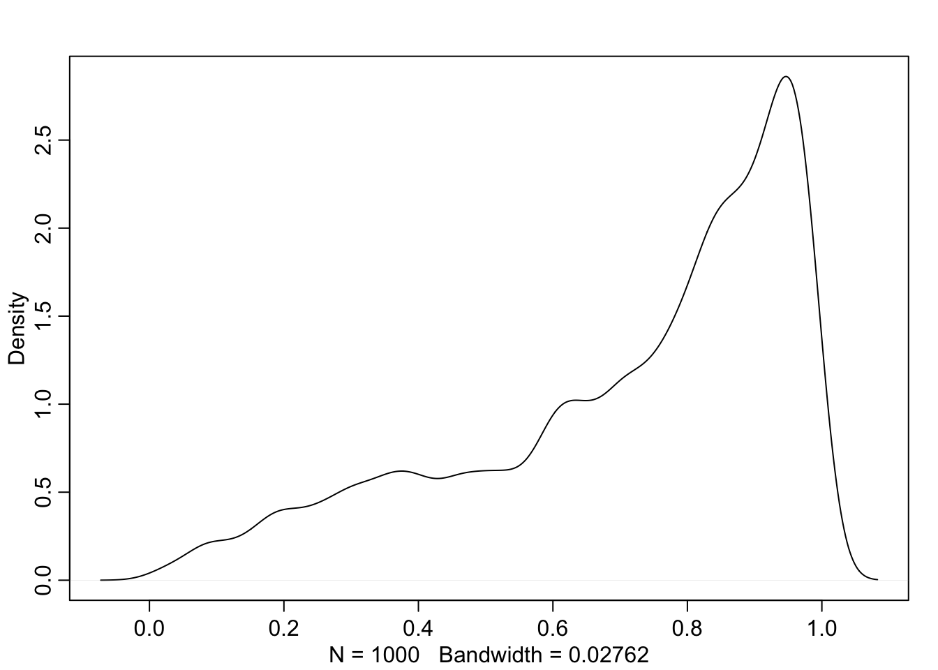
logistic_numbers %>% rethinking::HPDI(.)## |0.89 0.89|
## 0.3390388 0.99976885.1 The underfitting / overfitting tradeoff
a <- 1.4
sigma <- 1.5
nponds <- 60
ni <- rep(c(5L, 10L, 25L, 35L), each = nponds / 4)Simulate the ponds. In this example, ponds had the same chance of mortality, just different starting densities.
a_ponds <- rnorm(length(ni), mean = a, sd = sigma)
dsim <- data_frame(pond = seq_len(nponds),
ni = ni,
true_a = a_ponds)
simulated_observations <- dsim %>%
rowwise %>%
mutate(si = rbinom(1, prob = rethinking::logistic(true_a), size = ni),
#no-pooling estimate
p_nopool = si / ni)simulated_observations %>%
ggplot(aes(x = pond, y = p_nopool)) + geom_point() + facet_wrap(~ni)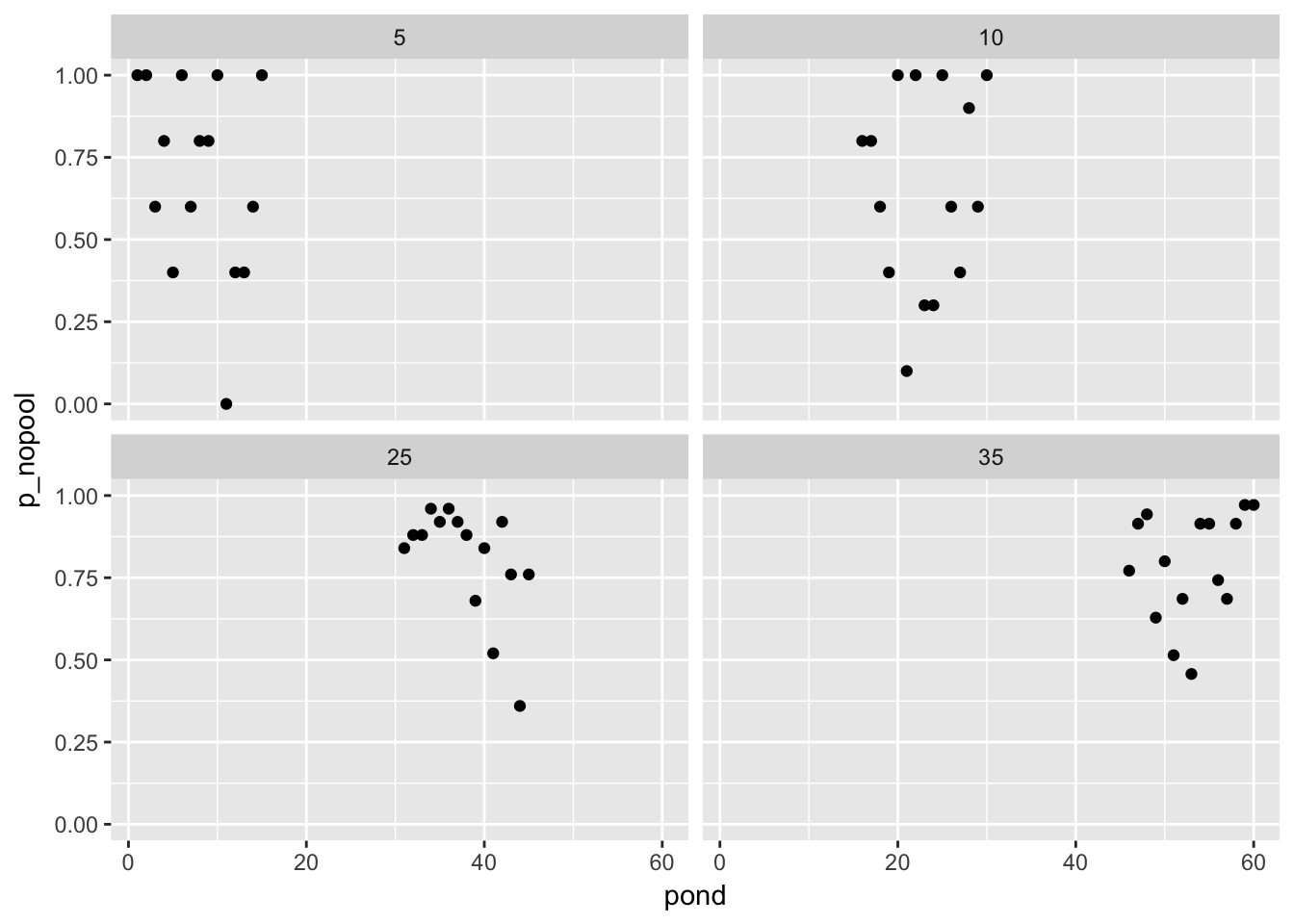
Now we have “fake observations” of the proportion of tadpoles who survived in each pond (we somehow have starting density? I guess we are simulating an experiment that has no density-dependent mortality).
## fit a model
model_12.3 <- alist(
si ~ dbinom(ni, p),
logit(p) <- a_pond[pond],
a_pond[pond] ~ dnorm(a, sigma),
a ~ dnorm(0, 1),
sigma ~ dcauchy(0,1)
)m12.3 <- rethinking::map2stan(
model_12.3,
data = as.data.frame(simulated_observations),
iter = 1e4, warmup = 1000
)
saveRDS(m12.3, file = "stan_models/m12.3.rds")m12.3 <- readRDS("stan_models/m12.3.rds")
rethinking::precis(m12.3, depth = 2)@output %>% head## Mean StdDev lower 0.89 upper 0.89 n_eff Rhat
## a_pond[1] 1.557822 0.8380886 0.2342690 2.868527 9000 1.0004711
## a_pond[2] 2.390155 0.9834414 0.8160344 3.900862 9000 0.9999574
## a_pond[3] 1.560175 0.8521043 0.1516030 2.866908 9000 0.9998903
## a_pond[4] 2.369144 0.9830625 0.7931416 3.871439 9000 1.0000201
## a_pond[5] 2.365656 0.9698000 0.8460757 3.911448 9000 1.0001061
## a_pond[6] 1.566072 0.8591920 0.2105865 2.941477 9000 0.9998890pooling_estimates <- rethinking::coef(m12.3) %>%
data_frame(coef = ., param = names(.)) %>%
filter(grepl("^a_pond", param)) %>%
mutate(p_partpool = rethinking::logistic(coef),
pond = readr::parse_number(param))
abs_error <- simulated_observations %>%
left_join(pooling_estimates, by = "pond") %>%
mutate(p_true = rethinking::logistic(true_a),
nopool_err = abs(p_nopool - p_true),
parpool_err = abs(p_partpool - p_true))abs_error %>%
ggplot(aes(x = p_true, y = p_nopool)) +
geom_point() +
geom_point(aes(y = p_partpool), fill = "red", pch = 21) +
geom_abline(slope = 1, intercept = 0) +
geom_hline(aes(yintercept = median(p_nopool))) +
geom_hline(aes(yintercept = median(p_partpool)), colour = "red")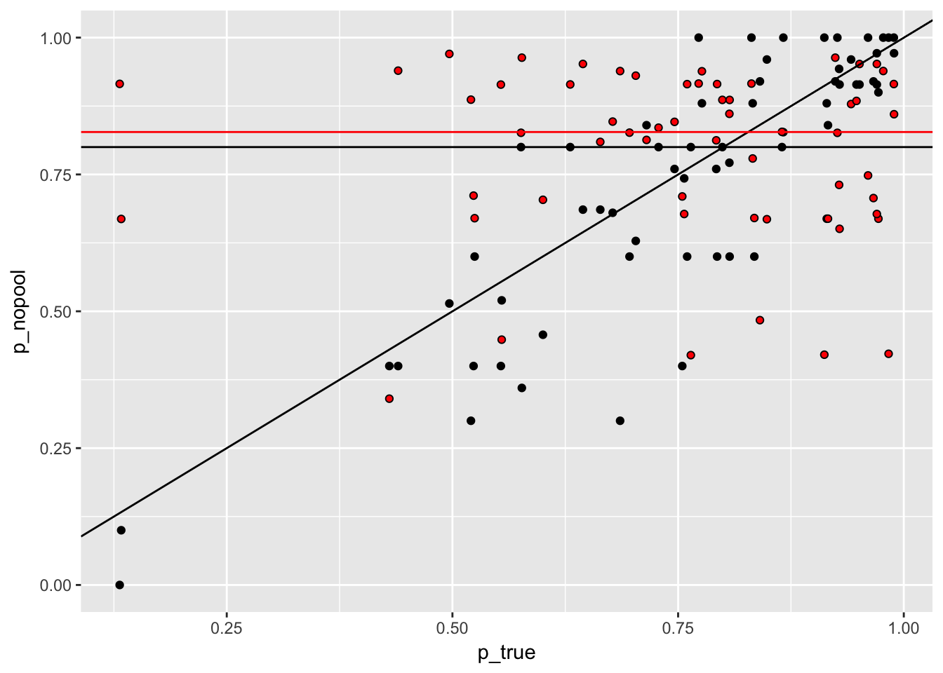
abs_error %>%
ungroup %>%
mutate(pond_rnk = dense_rank(abs(nopool_err - parpool_err))) %>%
ggplot(aes(x = pond_rnk, y = nopool_err)) +
geom_point() +
geom_point(aes(y = parpool_err), pch = 21, fill = "lightgrey") +
facet_wrap(~ni, scales = "free_x")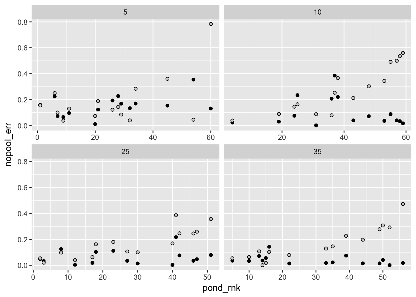
Ok so here, as in other cases, the regularizing prior shrinks parameters towards the median. By doing so, it also decreases the error (on average). In other words, models with regularizing priors would make better predictions – predictions which are closer to the true values.
5.2 More than one type of cluster
(how does this apply to bromeliad data? there we have both different intercepts for each species (i.e. each species having their own intercept values) and for bromeliads (each bromelaid having their own size). but might we not also want an observation-level intercept? one for every species x bromeliad count?)
data("chimpanzees", package = "rethinking")
chimpanzees %>% head %>% knitr::kable(.)| actor | recipient | condition | block | trial | prosoc_left | chose_prosoc | pulled_left |
|---|---|---|---|---|---|---|---|
| 1 | NA | 0 | 1 | 2 | 0 | 1 | 0 |
| 1 | NA | 0 | 1 | 4 | 0 | 0 | 1 |
| 1 | NA | 0 | 1 | 6 | 1 | 0 | 0 |
| 1 | NA | 0 | 1 | 8 | 0 | 1 | 0 |
| 1 | NA | 0 | 1 | 10 | 1 | 1 | 1 |
| 1 | NA | 0 | 1 | 12 | 1 | 1 | 1 |
multilevel_chimps <- alist(
pulled_left ~ dbinom(1, p),
logit(p) <- a + a_actor[actor] + (bp + bpC * condition) * prosoc_left,
a_actor[actor] ~ dnorm(0, sigma_actor),
a ~ dnorm(0, 10),
bp ~ dnorm(0, 10),
bpC ~ dnorm(0, 10),
sigma_actor ~ dcauchy(0, 1)
)m12.4 <- rethinking::map2stan(
multilevel_chimps,
data = chimpanzees %>% select(-recipient), warmup = 1000, iter = 5000, chains = 4, cores = 3)
saveRDS(m12.4, file = "stan_models/m12.4.rds")create the final distribution by sampling
m12.4 <- readRDS("stan_models/m12.4.rds")
samples_m12.4 <- rethinking::extract.samples(m12.4)
names(samples_m12.4)## [1] "a_actor" "a" "bp" "bpC" "sigma_actor"samples_m12.4 %>% map(head)## $a_actor
## [,1] [,2] [,3] [,4] [,5] [,6]
## [1,] -0.2498162 3.862380 -1.0615577 -1.5232305 -1.0719867 -0.1678776
## [2,] -0.4752955 3.182628 -0.6631407 -0.7949280 -0.4337731 0.5647808
## [3,] -0.6223943 3.481170 -1.0774757 -0.6951451 -0.1967038 0.5395006
## [4,] -1.1940592 2.149602 -1.5739781 -1.7122535 -1.4881367 -0.2527088
## [5,] -1.4561899 3.575433 -1.7670215 -2.0094237 -1.3636391 -0.3322763
## [6,] -1.4389213 3.670573 -1.5961623 -1.6164994 -0.9841400 -0.2458840
## [,7]
## [1,] 1.9920602
## [2,] 1.6186812
## [3,] 1.4089190
## [4,] 1.8642957
## [5,] 0.7073453
## [6,] 0.8283149
##
## $a
## [1] -0.2657715 -0.1103985 -0.1436957 0.5907273 0.7511017 0.2089818
##
## $bp
## [1] 0.9791574 0.4500455 0.5799394 0.9348228 1.0567673 1.2721056
##
## $bpC
## [1] 0.06038137 0.18105297 -0.08997335 -0.06034022 -0.41412474 -0.09969594
##
## $sigma_actor
## [1] 1.561006 1.417797 1.946058 1.719626 1.600610 1.843412with(samples_m12.4,
sweep(a_actor, 1, a, FUN = `+`)) %>%
colMeans## [1] -0.7158392 4.6322268 -1.0190221 -1.0224748 -0.7127088 0.2281226
## [7] 1.76108115.3 chimps with two kinds of cluster
Now we fit one for block (the chimps have “grabby days” and “less grabby days”) and also the chimps differ from each other. However, in each case, the relative effect of the two treatment variables is assumed to be the same.
m12.5 <- rethinking::map2stan(
alist(
pulled_left ~ dbinom(1, p),
logit(p) <- a + a_actor[actor] + a_block[block_id] +
(bp + bpc * condition) * prosoc_left,
a_actor[actor] ~ dnorm(0, sigma_actor),
a_block[block_id] ~ dnorm(0, sigma_block),
c(a, bpc, bp) ~ dnorm(0, 10),
sigma_actor ~ dcauchy(0, 1),
sigma_block ~ dcauchy(0, 1)
),
data = chimpanzees %>% rename(block_id = block),
warmup = 1000,
iter = 6000,
chains = 4,
cores = 3
)
saveRDS(m12.5, file = "stan_models/m12.5.rds")examining that model
m12.5 <- readRDS("stan_models/m12.5.rds")
m12.5_precis <- m12.5 %>% rethinking::precis(depth = 2)## Warning in rethinking::precis(., depth = 2): There were 47 divergent iterations during sampling.
## Check the chains (trace plots, n_eff, Rhat) carefully to ensure they are valid.m12.5_precis## Mean StdDev lower 0.89 upper 0.89 n_eff Rhat
## a_actor[1] -1.18 0.95 -2.65 0.25 3575 1
## a_actor[2] 4.16 1.65 1.83 6.37 5042 1
## a_actor[3] -1.49 0.95 -2.91 0.01 3624 1
## a_actor[4] -1.48 0.95 -2.98 -0.07 3583 1
## a_actor[5] -1.17 0.95 -2.62 0.27 3587 1
## a_actor[6] -0.23 0.95 -1.72 1.18 3625 1
## a_actor[7] 1.31 0.97 -0.12 2.84 3705 1
## a_block[1] -0.18 0.23 -0.55 0.11 3985 1
## a_block[2] 0.04 0.19 -0.24 0.34 10058 1
## a_block[3] 0.05 0.19 -0.22 0.36 9542 1
## a_block[4] 0.01 0.18 -0.27 0.31 11821 1
## a_block[5] -0.03 0.19 -0.32 0.26 10423 1
## a_block[6] 0.11 0.20 -0.16 0.44 6587 1
## a 0.46 0.94 -0.99 1.88 3502 1
## bpc -0.14 0.30 -0.63 0.33 12329 1
## bp 0.83 0.26 0.42 1.26 11825 1
## sigma_actor 2.27 0.92 1.04 3.40 5535 1
## sigma_block 0.22 0.18 0.01 0.43 2249 1#rethinking::plot(m12.5)
#what is this plot for??
plot(m12.5@stanfit)## 'pars' not specified. Showing first 10 parameters by default.## ci_level: 0.8 (80% intervals)## outer_level: 0.95 (95% intervals)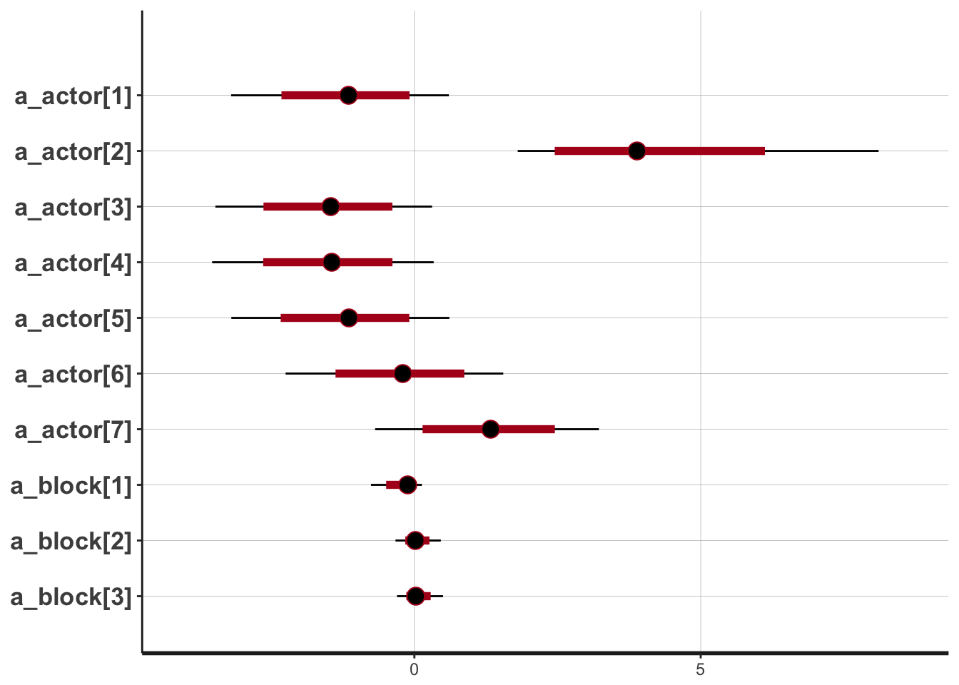
I can’t get any “real” trace plots to work!
plot(m12.5_precis)post <- rethinking::extract.samples(m12.5)
post %>%
.[c("sigma_actor", "sigma_block")] %>%
as.data.frame() %>%
tidyr::gather(param, value) %>%
ggplot(aes(x = value, fill = param)) + stat_density(alpha = 0.6) +
coord_cartesian(xlim = c(0, 5))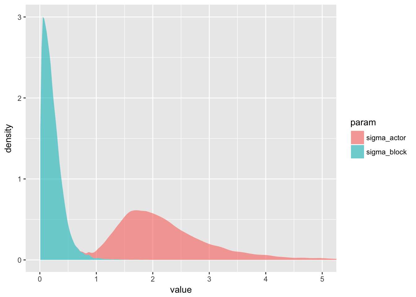
This is interesting because it shows that while the block effect is there, it really doesn’t matter much. So including it in the model has comparatively weak effects on the final results.
You can think of the
sigmaparameter for each cluster as a crude measure of the cluster’s relevance for explaining variation in the outcome.
That’s a rather powerful idea.
rethinking::compare(m12.4, m12.5)## WAIC pWAIC dWAIC weight SE dSE
## m12.4 531.4 8.1 0.0 0.65 19.49 NA
## m12.5 532.6 10.3 1.2 0.35 19.68 1.725.4 multilevel predictions
Two kinds of “prediction” can happen in a multilevel model (at least, a two-level one).
- Predictions for members of the same clusters
- Predictions for totally new clusters.
It seems to me that there are different variables, which might define clusters, which would be used in one or the other way. For example if we have data on insects in bromeliads, we might be interested in the future behaviour of these species, but not of these bromelaids.
Anyway.
Posterior predictions for chimpanzee model
d_pred_trts <- frame_data(
~prosoc_left, ~condition,
0, 0,
1, 0,
0, 1,
1, 1
)
test <- replicate(7, d_pred_trts, simplify = FALSE) %>%
bind_rows(.id = "actor") %>%
mutate(actor = as.numeric(actor)) %>%
select(prosoc_left, condition, actor)
link12.4 <- rethinking::link(m12.4, data = as.data.frame(test))## [ 100 / 1000 ]
[ 200 / 1000 ]
[ 300 / 1000 ]
[ 400 / 1000 ]
[ 500 / 1000 ]
[ 600 / 1000 ]
[ 700 / 1000 ]
[ 800 / 1000 ]
[ 900 / 1000 ]
[ 1000 / 1000 ]chimp_pred <- bind_cols(test,
link12.4 %>% apply(2, mean) %>% data_frame(m12.4_mean = .),
link12.4 %>% apply(2, rethinking::PI) %>% t %>% as.data.frame)
chimp_pred %>%
tidyr::unite("treatment", prosoc_left, condition) %>%
ggplot(aes(x = treatment,
y = m12.4_mean,
group = actor)) +
geom_ribbon(aes(ymax = `94%`, ymin = `5%`), fill = "forestgreen", alpha = 0.8) +
geom_point() +
geom_line()+
# coord_cartesian(ylim = c(0.5,1)) +
theme_minimal() +
facet_wrap(~actor)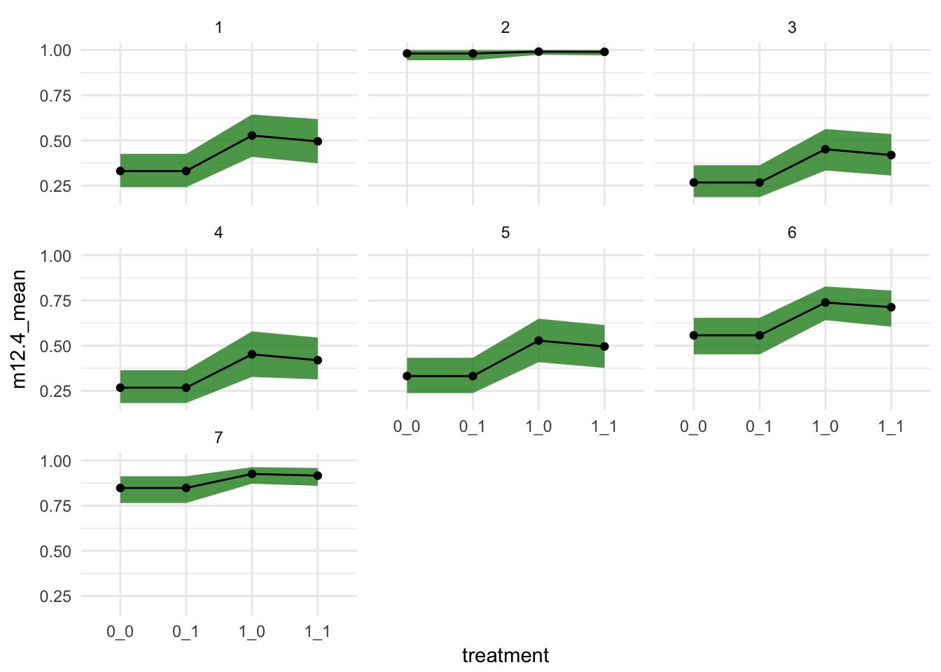
Now to try to do the same without link:
chimpanzees %>%
select(actor, block) %>%
group_by(actor, block) %>% tally## # A tibble: 42 x 3
## # Groups: actor [?]
## actor block n
## <int> <int> <int>
## 1 1 1 12
## 2 1 2 12
## 3 1 3 12
## 4 1 4 12
## 5 1 5 12
## 6 1 6 12
## 7 2 1 12
## 8 2 2 12
## 9 2 3 12
## 10 2 4 12
## # ... with 32 more rowswith(chimpanzees, table(actor, block))## block
## actor 1 2 3 4 5 6
## 1 12 12 12 12 12 12
## 2 12 12 12 12 12 12
## 3 12 12 12 12 12 12
## 4 12 12 12 12 12 12
## 5 12 12 12 12 12 12
## 6 12 12 12 12 12 12
## 7 12 12 12 12 12 12post <- rethinking::extract.samples(m12.4)
p_link <- function(prosoc_left, condition, actor){
logodds <- with(post,
a + a_actor[,actor] + (bp + bpC * condition) * prosoc_left)
rethinking::logistic(logodds)
}
test %>%
pmap(lift(p_link)) %>%
map_df(~ data_frame(pred_p = mean(.x),
pred_pi = list(rethinking::PI(.x)))) %>%
mutate(pred_low = map_dbl(pred_pi, 1),
pred_up = map_dbl(pred_pi, 2)) %>%
bind_cols(test,.) %>%
tidyr::unite("treatment", prosoc_left, condition) %>%
ggplot(aes(x = treatment,
y = pred_p,
group = actor)) +
geom_ribbon(aes(ymax = pred_up, ymin = pred_low), fill = "forestgreen", alpha = 0.8) +
geom_point() +
geom_line()+
# coord_cartesian(ylim = c(0.5,1)) +
theme_minimal() +
facet_wrap(~actor) +
geom_point(aes(y = pulled_left), data = chimpanzees %>%
tidyr::unite("treatment", prosoc_left, condition),
position = position_jitter(width = 0.1, height = 0.05), alpha = 0.3)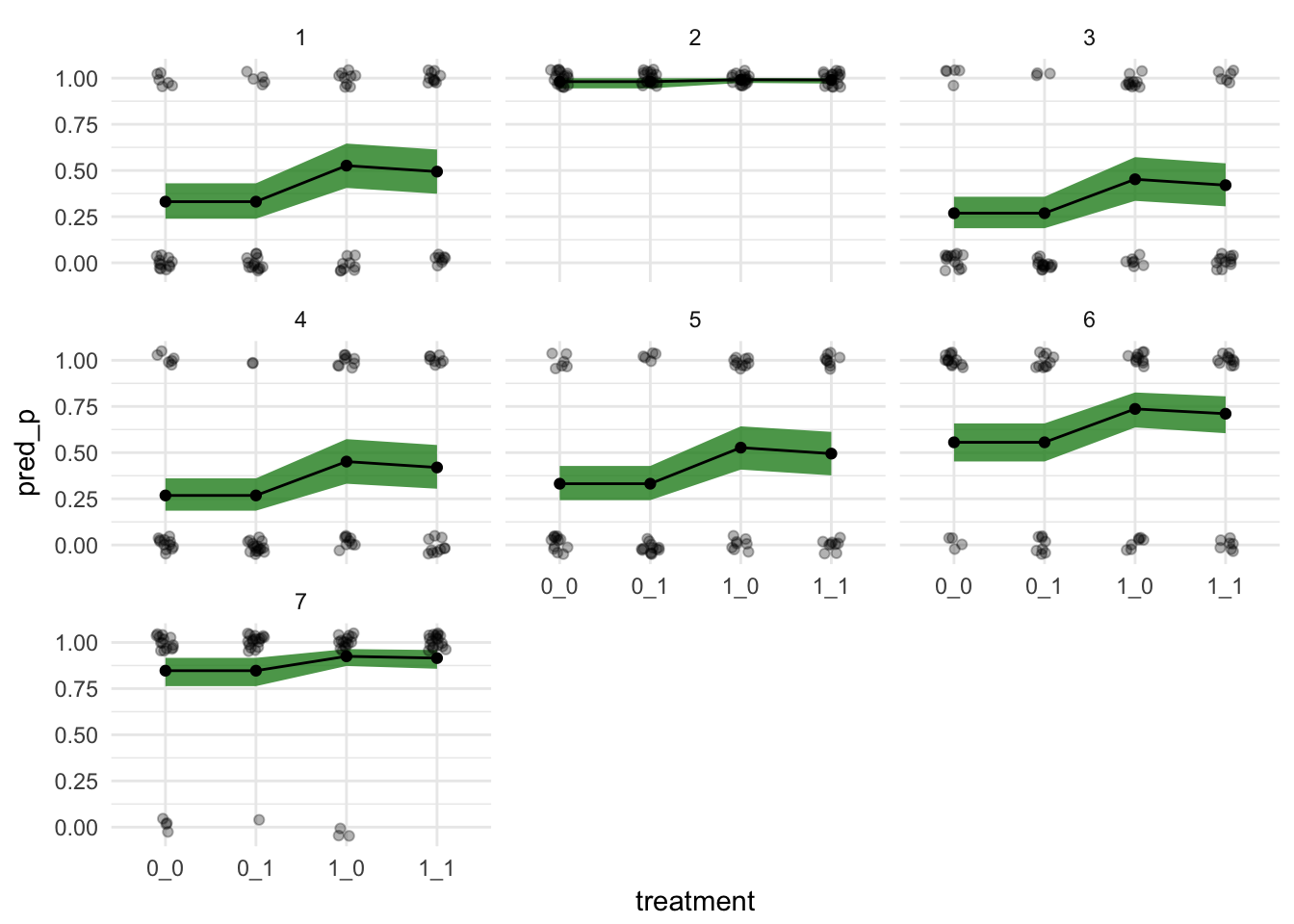
d_pred_trts <- frame_data(
~prosoc_left, ~condition,
0, 0,
1, 0,
0, 1,
1, 1
) %>%
mutate(actor = 2) # placeholder
a_actor_zeros <- matrix(0, 1000, 7)
link_m12.4_average <- rethinking::link(m12.4, n = 1000, data = d_pred_trts, replace = list(a_actor = a_actor_zeros))## [ 100 / 1000 ]
[ 200 / 1000 ]
[ 300 / 1000 ]
[ 400 / 1000 ]
[ 500 / 1000 ]
[ 600 / 1000 ]
[ 700 / 1000 ]
[ 800 / 1000 ]
[ 900 / 1000 ]
[ 1000 / 1000 ]bind_cols(d_pred_trts,
link_m12.4_average %>% apply(2, mean) %>% data_frame(m12.4_mean = .),
link_m12.4_average %>% apply(2, rethinking::PI) %>% t %>% as.data.frame) %>%
tidyr::unite("treatment", prosoc_left, condition) %>%
ggplot(aes(x = treatment,
y = m12.4_mean,
group = actor)) +
geom_ribbon(aes(ymax = `94%`, ymin = `5%`), fill = "forestgreen", alpha = 0.8) +
geom_point() +
geom_line()+
coord_cartesian(ylim = c(0,1)) +
theme_minimal() +
facet_wrap(~actor)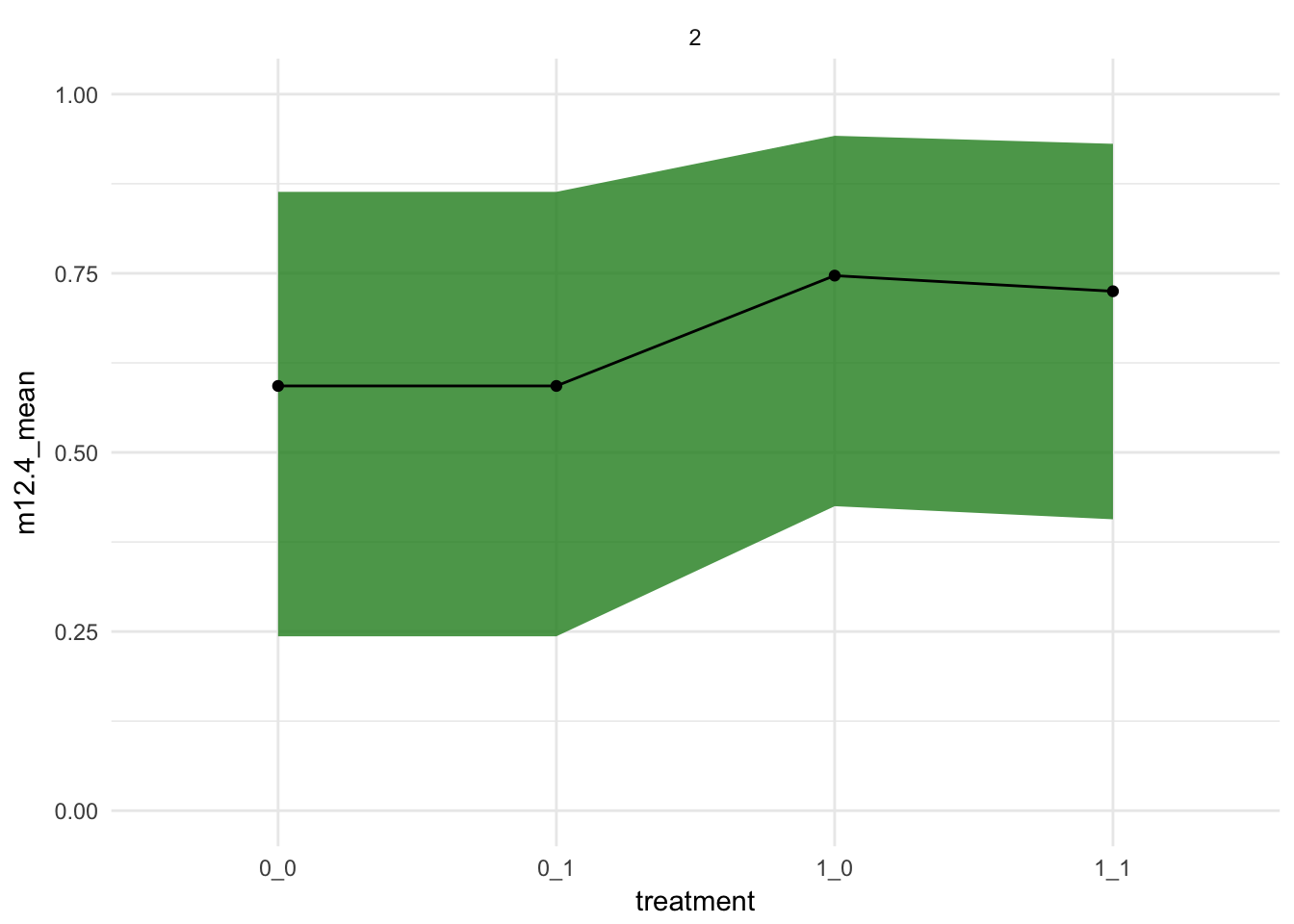
post <- rethinking::extract.samples(m12.4)
map(post, head)## $a_actor
## [,1] [,2] [,3] [,4] [,5] [,6]
## [1,] -0.2498162 3.862380 -1.0615577 -1.5232305 -1.0719867 -0.1678776
## [2,] -0.4752955 3.182628 -0.6631407 -0.7949280 -0.4337731 0.5647808
## [3,] -0.6223943 3.481170 -1.0774757 -0.6951451 -0.1967038 0.5395006
## [4,] -1.1940592 2.149602 -1.5739781 -1.7122535 -1.4881367 -0.2527088
## [5,] -1.4561899 3.575433 -1.7670215 -2.0094237 -1.3636391 -0.3322763
## [6,] -1.4389213 3.670573 -1.5961623 -1.6164994 -0.9841400 -0.2458840
## [,7]
## [1,] 1.9920602
## [2,] 1.6186812
## [3,] 1.4089190
## [4,] 1.8642957
## [5,] 0.7073453
## [6,] 0.8283149
##
## $a
## [1] -0.2657715 -0.1103985 -0.1436957 0.5907273 0.7511017 0.2089818
##
## $bp
## [1] 0.9791574 0.4500455 0.5799394 0.9348228 1.0567673 1.2721056
##
## $bpC
## [1] 0.06038137 0.18105297 -0.08997335 -0.06034022 -0.41412474 -0.09969594
##
## $sigma_actor
## [1] 1.561006 1.417797 1.946058 1.719626 1.600610 1.843412sim_actor <- function(a, bp, bpC, sigma_actor){
# 'random' effects
sim_a_actor <- rnorm(1, 0, sd = sigma_actor)
# 'fixed' effects
P <- c(0, 1, 0, 1)
C <- c(0, 0, 1, 1)
p <- a + sim_a_actor + (bp + bpC * C) * P
return(rethinking::logistic(p))
}
simulated_actors <- post %>%
# drop the matrix of random effects
discard(is.matrix) %>%
as.data.frame %>%
pmap(lift(sim_actor))
simulated_df <- simulated_actors %>%
map_df(~data_frame(
P = c(0, 1, 0, 1),
C = c(0, 0, 1, 1),
p_resp = .x
), .id = "sim")
points_lines <- simulated_df %>%
filter(sim %in% sample(1:1600, size = 800, replace = FALSE)) %>%
tidyr::unite("treatment", P, C) %>%
ggplot(aes(x = treatment, y = p_resp, group = sim)) +
# geom_point(alpha = 0.002)+
geom_line(alpha = 0.1) +
theme_classic()
points_lines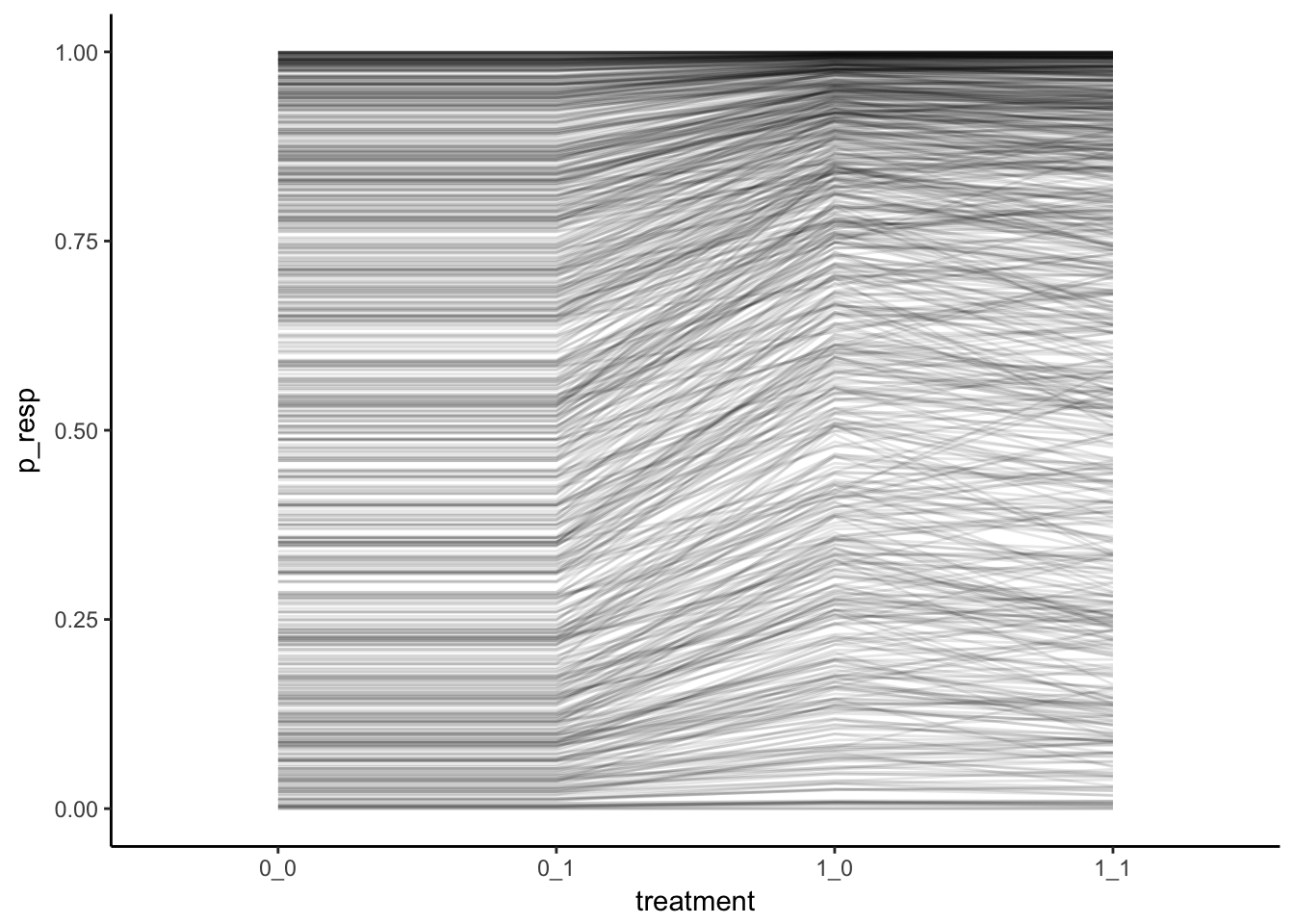
5.5 varying intercepts to model over-dispersion
you can model over-dispersion by modelling a random intercept for every observation. This i suppose is like adding an offset term?
data("Kline", package = "rethinking")
Kline## culture population contact total_tools mean_TU
## 1 Malekula 1100 low 13 3.2
## 2 Tikopia 1500 low 22 4.7
## 3 Santa Cruz 3600 low 24 4.0
## 4 Yap 4791 high 43 5.0
## 5 Lau Fiji 7400 high 33 5.0
## 6 Trobriand 8000 high 19 4.0
## 7 Chuuk 9200 high 40 3.8
## 8 Manus 13000 low 28 6.6
## 9 Tonga 17500 high 55 5.4
## 10 Hawaii 275000 low 71 6.6kline_formodel <- Kline %>%
mutate(logpop = log(population)) %>%
tibble::rownames_to_column("society")
varying_intercepts <- alist(
total_tools ~ dpois(mu),
log(mu) <- a + a_society[society] + bp * logpop,
a ~ dnorm(0, 10),
bp ~ dnorm(0, 1),
a_society[society] ~ dnorm(0, sigma_society),
sigma_society ~ dcauchy(0, 1)
)m12.6 <- rethinking::map2stan(varying_intercepts,
data = as.data.frame(kline_formodel %>%
mutate(society = as.numeric(society))),
iter = 4000, chains = 3)## In file included from file107514afae61.cpp:8:
## In file included from /Library/Frameworks/R.framework/Versions/3.4/Resources/library/StanHeaders/include/src/stan/model/model_header.hpp:4:
## In file included from /Library/Frameworks/R.framework/Versions/3.4/Resources/library/StanHeaders/include/stan/math.hpp:4:
## In file included from /Library/Frameworks/R.framework/Versions/3.4/Resources/library/StanHeaders/include/stan/math/rev/mat.hpp:4:
## In file included from /Library/Frameworks/R.framework/Versions/3.4/Resources/library/StanHeaders/include/stan/math/rev/core.hpp:12:
## In file included from /Library/Frameworks/R.framework/Versions/3.4/Resources/library/StanHeaders/include/stan/math/rev/core/gevv_vvv_vari.hpp:5:
## In file included from /Library/Frameworks/R.framework/Versions/3.4/Resources/library/StanHeaders/include/stan/math/rev/core/var.hpp:7:
## In file included from /Library/Frameworks/R.framework/Versions/3.4/Resources/library/BH/include/boost/math/tools/config.hpp:13:
## In file included from /Library/Frameworks/R.framework/Versions/3.4/Resources/library/BH/include/boost/config.hpp:39:
## /Library/Frameworks/R.framework/Versions/3.4/Resources/library/BH/include/boost/config/compiler/clang.hpp:200:11: warning: 'BOOST_NO_CXX11_RVALUE_REFERENCES' macro redefined [-Wmacro-redefined]
## # define BOOST_NO_CXX11_RVALUE_REFERENCES
## ^
## <command line>:6:9: note: previous definition is here
## #define BOOST_NO_CXX11_RVALUE_REFERENCES 1
## ^
## 1 warning generated.
##
## SAMPLING FOR MODEL 'total_tools ~ dpois(mu)' NOW (CHAIN 1).
##
## Gradient evaluation took 2.8e-05 seconds
## 1000 transitions using 10 leapfrog steps per transition would take 0.28 seconds.
## Adjust your expectations accordingly!
##
##
## Iteration: 1 / 4000 [ 0%] (Warmup)
## Iteration: 400 / 4000 [ 10%] (Warmup)
## Iteration: 800 / 4000 [ 20%] (Warmup)
## Iteration: 1200 / 4000 [ 30%] (Warmup)
## Iteration: 1600 / 4000 [ 40%] (Warmup)
## Iteration: 2000 / 4000 [ 50%] (Warmup)
## Iteration: 2001 / 4000 [ 50%] (Sampling)
## Iteration: 2400 / 4000 [ 60%] (Sampling)
## Iteration: 2800 / 4000 [ 70%] (Sampling)
## Iteration: 3200 / 4000 [ 80%] (Sampling)
## Iteration: 3600 / 4000 [ 90%] (Sampling)
## Iteration: 4000 / 4000 [100%] (Sampling)
##
## Elapsed Time: 0.490841 seconds (Warm-up)
## 0.644079 seconds (Sampling)
## 1.13492 seconds (Total)
##
##
## SAMPLING FOR MODEL 'total_tools ~ dpois(mu)' NOW (CHAIN 2).
##
## Gradient evaluation took 1.9e-05 seconds
## 1000 transitions using 10 leapfrog steps per transition would take 0.19 seconds.
## Adjust your expectations accordingly!
##
##
## Iteration: 1 / 4000 [ 0%] (Warmup)
## Iteration: 400 / 4000 [ 10%] (Warmup)
## Iteration: 800 / 4000 [ 20%] (Warmup)
## Iteration: 1200 / 4000 [ 30%] (Warmup)
## Iteration: 1600 / 4000 [ 40%] (Warmup)
## Iteration: 2000 / 4000 [ 50%] (Warmup)
## Iteration: 2001 / 4000 [ 50%] (Sampling)
## Iteration: 2400 / 4000 [ 60%] (Sampling)
## Iteration: 2800 / 4000 [ 70%] (Sampling)
## Iteration: 3200 / 4000 [ 80%] (Sampling)
## Iteration: 3600 / 4000 [ 90%] (Sampling)
## Iteration: 4000 / 4000 [100%] (Sampling)
##
## Elapsed Time: 0.515647 seconds (Warm-up)
## 0.781854 seconds (Sampling)
## 1.2975 seconds (Total)
##
##
## SAMPLING FOR MODEL 'total_tools ~ dpois(mu)' NOW (CHAIN 3).
##
## Gradient evaluation took 1.2e-05 seconds
## 1000 transitions using 10 leapfrog steps per transition would take 0.12 seconds.
## Adjust your expectations accordingly!
##
##
## Iteration: 1 / 4000 [ 0%] (Warmup)
## Iteration: 400 / 4000 [ 10%] (Warmup)
## Iteration: 800 / 4000 [ 20%] (Warmup)
## Iteration: 1200 / 4000 [ 30%] (Warmup)
## Iteration: 1600 / 4000 [ 40%] (Warmup)
## Iteration: 2000 / 4000 [ 50%] (Warmup)
## Iteration: 2001 / 4000 [ 50%] (Sampling)
## Iteration: 2400 / 4000 [ 60%] (Sampling)
## Iteration: 2800 / 4000 [ 70%] (Sampling)
## Iteration: 3200 / 4000 [ 80%] (Sampling)
## Iteration: 3600 / 4000 [ 90%] (Sampling)
## Iteration: 4000 / 4000 [100%] (Sampling)
##
## Elapsed Time: 0.677524 seconds (Warm-up)
## 0.548449 seconds (Sampling)
## 1.22597 seconds (Total)
##
##
## SAMPLING FOR MODEL 'total_tools ~ dpois(mu)' NOW (CHAIN 1).
##
## Gradient evaluation took 7e-06 seconds
## 1000 transitions using 10 leapfrog steps per transition would take 0.07 seconds.
## Adjust your expectations accordingly!
##
##
## WARNING: No variance estimation is
## performed for num_warmup < 20
##
## Iteration: 1 / 1 [100%] (Sampling)
##
## Elapsed Time: 0 seconds (Warm-up)
## 2.6e-05 seconds (Sampling)
## 2.6e-05 seconds (Total)## Warning: There were 1 divergent transitions after warmup. Increasing adapt_delta above 0.8 may help. See
## http://mc-stan.org/misc/warnings.html#divergent-transitions-after-warmup## Warning: Examine the pairs() plot to diagnose sampling problems## Computing WAIC## Constructing posterior predictions## [ 600 / 6000 ]
[ 1200 / 6000 ]
[ 1800 / 6000 ]
[ 2400 / 6000 ]
[ 3000 / 6000 ]
[ 3600 / 6000 ]
[ 4200 / 6000 ]
[ 4800 / 6000 ]
[ 5400 / 6000 ]
[ 6000 / 6000 ]saveRDS(m12.6, "stan_models/m12.6.rds")Checking this model out:
rethinking::WAIC(m12.6)## [1] 70.16342
## attr(,"lppd")
## [1] -30.02394
## attr(,"pWAIC")
## [1] 5.057768
## attr(,"se")
## [1] 2.426204Just to see, how does it compare to the constant intercept model:
constant_intercepts <- alist(
total_tools ~ dpois(mu),
log(mu) <- a + bp * logpop,
a ~ dnorm(0, 100),
bp ~ dnorm(0, 1)
)
m12.7 <- rethinking::map2stan(constant_intercepts,
data = as.data.frame(kline_formodel %>%
mutate(society = as.numeric(society))),)## In file included from file1075580acd14.cpp:8:
## In file included from /Library/Frameworks/R.framework/Versions/3.4/Resources/library/StanHeaders/include/src/stan/model/model_header.hpp:4:
## In file included from /Library/Frameworks/R.framework/Versions/3.4/Resources/library/StanHeaders/include/stan/math.hpp:4:
## In file included from /Library/Frameworks/R.framework/Versions/3.4/Resources/library/StanHeaders/include/stan/math/rev/mat.hpp:4:
## In file included from /Library/Frameworks/R.framework/Versions/3.4/Resources/library/StanHeaders/include/stan/math/rev/core.hpp:12:
## In file included from /Library/Frameworks/R.framework/Versions/3.4/Resources/library/StanHeaders/include/stan/math/rev/core/gevv_vvv_vari.hpp:5:
## In file included from /Library/Frameworks/R.framework/Versions/3.4/Resources/library/StanHeaders/include/stan/math/rev/core/var.hpp:7:
## In file included from /Library/Frameworks/R.framework/Versions/3.4/Resources/library/BH/include/boost/math/tools/config.hpp:13:
## In file included from /Library/Frameworks/R.framework/Versions/3.4/Resources/library/BH/include/boost/config.hpp:39:
## /Library/Frameworks/R.framework/Versions/3.4/Resources/library/BH/include/boost/config/compiler/clang.hpp:200:11: warning: 'BOOST_NO_CXX11_RVALUE_REFERENCES' macro redefined [-Wmacro-redefined]
## # define BOOST_NO_CXX11_RVALUE_REFERENCES
## ^
## <command line>:6:9: note: previous definition is here
## #define BOOST_NO_CXX11_RVALUE_REFERENCES 1
## ^
## 1 warning generated.
##
## SAMPLING FOR MODEL 'total_tools ~ dpois(mu)' NOW (CHAIN 1).
##
## Gradient evaluation took 1.1e-05 seconds
## 1000 transitions using 10 leapfrog steps per transition would take 0.11 seconds.
## Adjust your expectations accordingly!
##
##
## Iteration: 1 / 2000 [ 0%] (Warmup)
## Iteration: 200 / 2000 [ 10%] (Warmup)
## Iteration: 400 / 2000 [ 20%] (Warmup)
## Iteration: 600 / 2000 [ 30%] (Warmup)
## Iteration: 800 / 2000 [ 40%] (Warmup)
## Iteration: 1000 / 2000 [ 50%] (Warmup)
## Iteration: 1001 / 2000 [ 50%] (Sampling)
## Iteration: 1200 / 2000 [ 60%] (Sampling)
## Iteration: 1400 / 2000 [ 70%] (Sampling)
## Iteration: 1600 / 2000 [ 80%] (Sampling)
## Iteration: 1800 / 2000 [ 90%] (Sampling)
## Iteration: 2000 / 2000 [100%] (Sampling)
##
## Elapsed Time: 0.043282 seconds (Warm-up)
## 0.050789 seconds (Sampling)
## 0.094071 seconds (Total)
##
##
## SAMPLING FOR MODEL 'total_tools ~ dpois(mu)' NOW (CHAIN 1).
##
## Gradient evaluation took 6e-06 seconds
## 1000 transitions using 10 leapfrog steps per transition would take 0.06 seconds.
## Adjust your expectations accordingly!
##
##
## WARNING: No variance estimation is
## performed for num_warmup < 20
##
## Iteration: 1 / 1 [100%] (Sampling)
##
## Elapsed Time: 1e-06 seconds (Warm-up)
## 1.9e-05 seconds (Sampling)
## 2e-05 seconds (Total)## Warning: There were 1 divergent transitions after warmup. Increasing adapt_delta above 0.8 may help. See
## http://mc-stan.org/misc/warnings.html#divergent-transitions-after-warmup## Warning: Examine the pairs() plot to diagnose sampling problems## Computing WAIC## Constructing posterior predictions## [ 100 / 1000 ]
[ 200 / 1000 ]
[ 300 / 1000 ]
[ 400 / 1000 ]
[ 500 / 1000 ]
[ 600 / 1000 ]
[ 700 / 1000 ]
[ 800 / 1000 ]
[ 900 / 1000 ]
[ 1000 / 1000 ]saveRDS(m12.7, "stan_models/m12.7.rds")par(mfrow = c(1, 2))
rethinking::postcheck(m12.6)## [ 100 / 1000 ]
[ 200 / 1000 ]
[ 300 / 1000 ]
[ 400 / 1000 ]
[ 500 / 1000 ]
[ 600 / 1000 ]
[ 700 / 1000 ]
[ 800 / 1000 ]
[ 900 / 1000 ]
[ 1000 / 1000 ]
## [ 100 / 1000 ]
[ 200 / 1000 ]
[ 300 / 1000 ]
[ 400 / 1000 ]
[ 500 / 1000 ]
[ 600 / 1000 ]
[ 700 / 1000 ]
[ 800 / 1000 ]
[ 900 / 1000 ]
[ 1000 / 1000 ]rethinking::postcheck(m12.7)## [ 100 / 1000 ]
[ 200 / 1000 ]
[ 300 / 1000 ]
[ 400 / 1000 ]
[ 500 / 1000 ]
[ 600 / 1000 ]
[ 700 / 1000 ]
[ 800 / 1000 ]
[ 900 / 1000 ]
[ 1000 / 1000 ]
## [ 100 / 1000 ]
[ 200 / 1000 ]
[ 300 / 1000 ]
[ 400 / 1000 ]
[ 500 / 1000 ]
[ 600 / 1000 ]
[ 700 / 1000 ]
[ 800 / 1000 ]
[ 900 / 1000 ]
[ 1000 / 1000 ]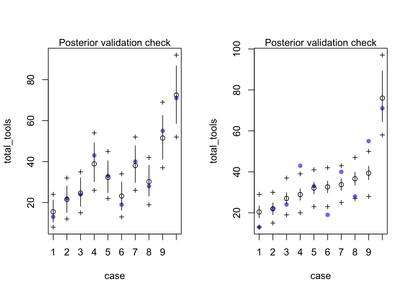
rethinking::compare(m12.6, m12.7)## WAIC pWAIC dWAIC weight SE dSE
## m12.6 70.2 5.1 0.0 1 2.43 NA
## m12.7 84.0 3.5 13.8 0 8.87 7.4post_m12.6 <- rethinking::extract.samples(m12.6)
d_predictions <- kline_formodel %>%
modelr::data_grid(logpop = modelr::seq_range(logpop, n = 30, expand = TRUE)) %>%
mutate(society = 1)
a_society_sims <- rnorm(2e4, 0, post_m12.6$sigma_society)
a_society_sims <- matrix(a_society_sims, ncol = 10)
link_m12.6 <- rethinking::link(m12.6, n= 2000, data = d_predictions,
replace = list(a_society=a_society_sims))## [ 200 / 2000 ]
[ 400 / 2000 ]
[ 600 / 2000 ]
[ 800 / 2000 ]
[ 1000 / 2000 ]
[ 1200 / 2000 ]
[ 1400 / 2000 ]
[ 1600 / 2000 ]
[ 1800 / 2000 ]
[ 2000 / 2000 ]link_m12.6 %>% head## [,1] [,2] [,3] [,4] [,5] [,6] [,7]
## [1,] 6.304190 6.975963 7.719319 8.541888 9.452109 10.45932 11.57387
## [2,] 8.047938 8.803966 9.631016 10.535760 11.525496 12.60821 13.79263
## [3,] 13.982838 15.048257 16.194854 17.428817 18.756801 20.18597 21.72403
## [4,] 9.108725 10.125233 11.255179 12.511225 13.907442 15.45947 17.18471
## [5,] 82.599645 81.909845 81.225806 80.547480 79.874818 79.20777 78.54630
## [6,] 10.930166 12.459757 14.203402 16.191057 18.456868 21.03976 23.98411
## [,8] [,9] [,10] [,11] [,12] [,13] [,14]
## [1,] 12.80717 14.17190 15.68206 17.35313 19.20228 21.24847 23.51270
## [2,] 15.08832 16.50572 18.05628 19.75250 21.60806 23.63794 25.85850
## [3,] 23.37929 25.16067 27.07778 29.14096 31.36135 33.75092 36.32256
## [4,] 19.10247 21.23425 23.60393 26.23806 29.16616 32.42102 36.03911
## [5,] 77.89035 77.23988 76.59484 75.95519 75.32087 74.69186 74.06810
## [6,] 27.34050 31.16659 35.52811 40.49999 46.16765 52.62845 59.99338
## [,15] [,16] [,17] [,18] [,19] [,20] [,21]
## [1,] 26.01820 28.79070 31.85863 35.25347 39.01007 43.16698 47.76684
## [2,] 28.28766 30.94502 33.85202 37.03210 40.51091 44.31654 48.47966
## [3,] 39.09015 42.06861 45.27402 48.72366 52.43614 56.43150 60.73128
## [4,] 40.06097 44.53166 49.50126 55.02546 61.16615 67.99211 75.57984
## [5,] 73.44955 72.83616 72.22790 71.62471 71.02657 70.43342 69.84522
## [6,] 68.38899 77.95949 88.86931 101.30587 115.48284 131.64375 150.06626
## [,22] [,23] [,24] [,25] [,26] [,27] [,28]
## [1,] 52.85686 58.48927 64.72187 71.61862 79.25027 87.69516 97.03993
## [2,] 53.03387 58.01590 63.46595 69.42798 75.95009 83.08488 90.88993
## [3,] 65.35869 70.33867 75.69811 81.46590 87.67317 94.35341 101.54264
## [4,] 84.01433 93.39009 103.81216 115.39730 128.27530 142.59046 158.50315
## [5,] 69.26193 68.68352 68.10993 67.54114 66.97709 66.41776 65.86310
## [6,] 171.06686 195.00633 222.29594 253.40451 288.86648 329.29108 375.37279
## [,29] [,30]
## [1,] 107.38048 118.82292
## [2,] 99.42818 108.76853
## [3,] 109.27965 117.60618
## [4,] 176.19164 195.85413
## [5,] 65.31307 64.76763
## [6,] 427.90327 487.78498plotting
col_pi <- partial(apply, MARGIN = 2, FUN = rethinking::PI)

col_pi(link_m12.6, prob = 0.62)
## [,1] [,2] [,3] [,4] [,5] [,6] [,7]
## 19% 5.897166 6.593443 7.455628 8.371946 9.465122 10.55556 11.86066
## 81% 13.824574 15.004626 16.268039 17.616715 19.035919 20.83796 22.74603
## [,8] [,9] [,10] [,11] [,12] [,13] [,14]
## 19% 13.19432 14.76736 16.63356 18.60554 20.60924 22.87300 25.12454
## 81% 24.73148 27.12311 29.61256 32.49679 35.64552 39.21192 43.14677
## [,15] [,16] [,17] [,18] [,19] [,20] [,21]
## 19% 27.69002 30.35720 33.23063 36.20844 39.35330 42.83805 47.11832
## 81% 47.62252 52.81244 58.69931 65.18903 72.78758 81.84589 91.02000
## [,22] [,23] [,24] [,25] [,26] [,27] [,28]
## 19% 51.27306 55.68837 60.60081 65.63009 70.65164 76.67306 82.35189
## 81% 102.42504 115.64579 129.51013 144.60682 162.87745 182.76990 205.12656
## [,29] [,30]
## 19% 88.46753 95.18318
## 81% 231.54846 260.41068shades <- viridisLite::viridis(3, end = 0.4, alpha = 0.8)
tool_plot <- bind_cols(d_predictions,
link_m12.6 %>% apply(2, mean) %>% data_frame(m12.4_mean = .),
link_m12.6 %>% col_pi(prob = 0.97) %>% t %>% as.data.frame,
link_m12.6 %>% col_pi(prob = 0.89) %>% t %>% as.data.frame,
link_m12.6 %>% col_pi(prob = 0.67) %>% t %>% as.data.frame) %>%
ggplot(aes(x = logpop, ymin = `2%`, ymax = `98%`)) +
geom_ribbon(fill = shades[1]) +
geom_ribbon(aes(ymin = `5%`, ymax = `94%`), fill = shades[2]) +
geom_ribbon(aes(ymin = `16%`, ymax = `84%`), fill = shades[3]) +
theme_bw() +
geom_point(aes(y = total_tools, ymin = NULL, ymax = NULL),
shape = 21, fill = "lightgrey", data = kline_formodel, stroke = 1.3, size = 2)
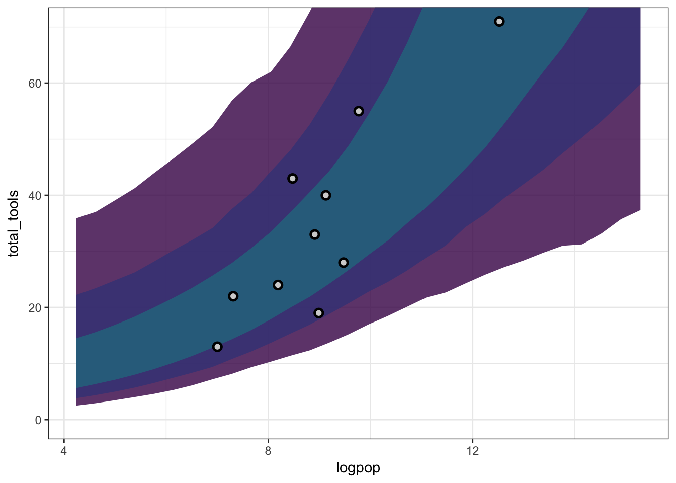
tool_plot + coord_cartesian(ylim = c(0, 70))