Chapter 2 Small worlds and large worlds

This chapter invites us to vary the probability of a binomial trial, in which we have 6 successes in 9 trials. Let’s just do it all at once:

curve(dbinom(6, size= 9, prob = x))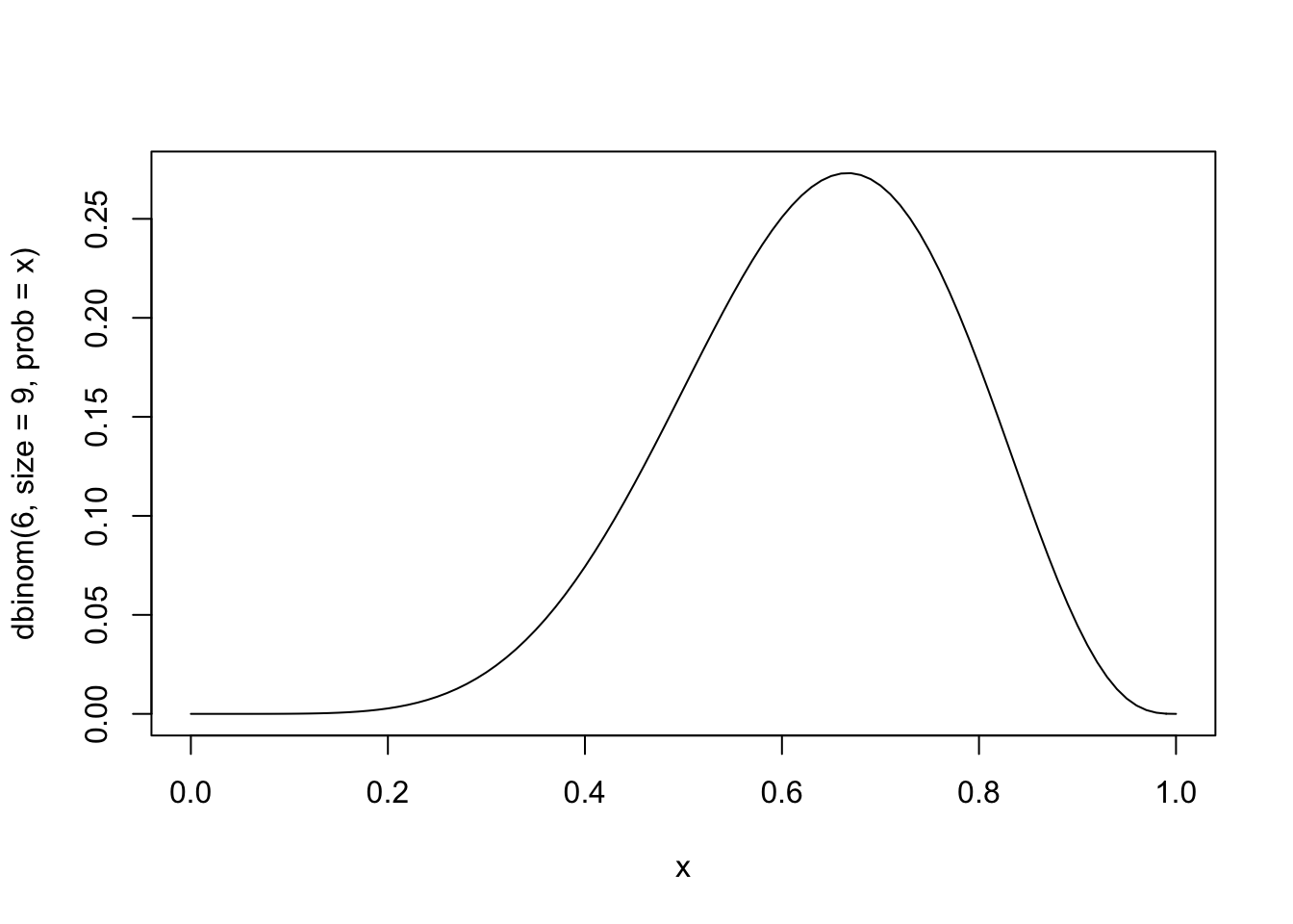

should’t the peak of that curve be right at \(6/9\)?

curve(dbinom(6, size= 9, prob = x))
abline(v = 6/9)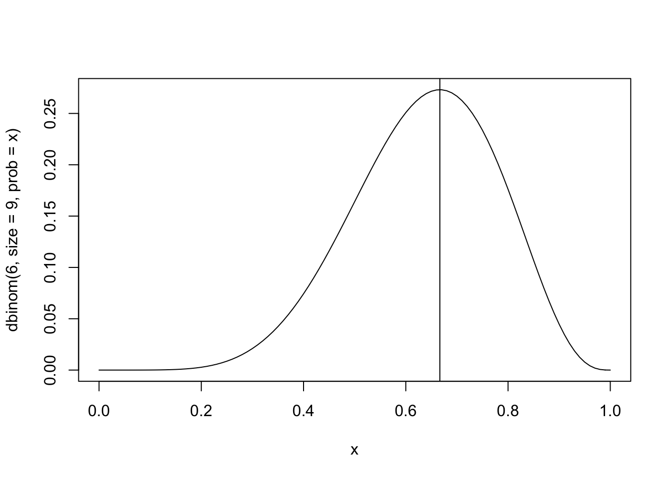

neat.

2.1 reproducing figures in text

d <- data_frame(p_grid          = seq(from = 0, to = 1, length.out = 200),
                prior           = 1,
                likelihood      = dbinom(6, size = 9, prob = p_grid),
                unstd.posterior = likelihood * prior,
                posterior       = unstd.posterior / sum(unstd.posterior))

knitr::kable(head(d))

p_grid	prior	likelihood	unstd.posterior	posterior
0.0000000	1	0	0	0
0.0050251	1	0	0	0
0.0100503	1	0	0	0
0.0150754	1	0	0	0
0.0201005	1	0	0	0
0.0251256	1	0	0	0

and a little plot:

post_plot <- d %>% 
  ggplot(aes(x = p_grid, y = posterior)) + 
  geom_point() + 
  geom_line() + 
  theme_light() +
  geom_vline(xintercept = 6/9) +
  labs(x = "probability of water", y = "Posterior probability")

print(post_plot)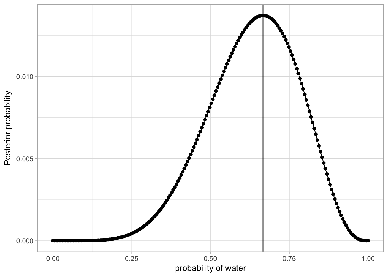

isn’t that.. exactly the probability density?

post_plot +
  stat_function(fun = function(x) dbinom(6, size= 9, prob = x))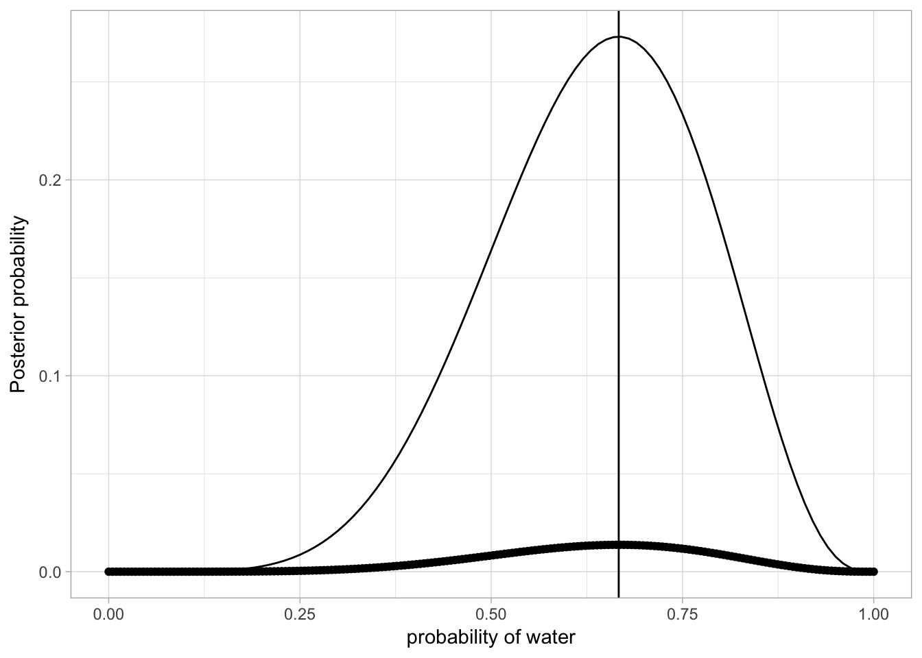

Whoops no.

2.1.1 with various priors

## a grid-approximating function -- that takes a "prior making function" as input

make_grid_approx <- function(f){
  data_frame(p_grid          = seq(from = 0, to = 1, length.out = 200),
             prior           = f(p_grid),
             likelihood      = dbinom(6, size = 9, prob = p_grid),
             unstd.posterior = likelihood * prior,
             posterior       = unstd.posterior / sum(unstd.posterior))
}



list(constant = function(x) 1,
     steppy = function(x) ifelse(x < 0.5, 0, 1),
     pointy = function(x) exp(-5 * abs(x - 0.5))) %>% 
  map(make_grid_approx) %>% 
  bind_rows(.id = "prior_shape") %>%  
  ggplot(aes(x = p_grid, y = posterior)) + 
  geom_point() + 
  geom_line() + 
  theme_light() +
  geom_vline(xintercept = 6/9) +
  labs(x = "probability of water", y = "Posterior probability") +
  facet_wrap(~prior_shape, ncol = 1)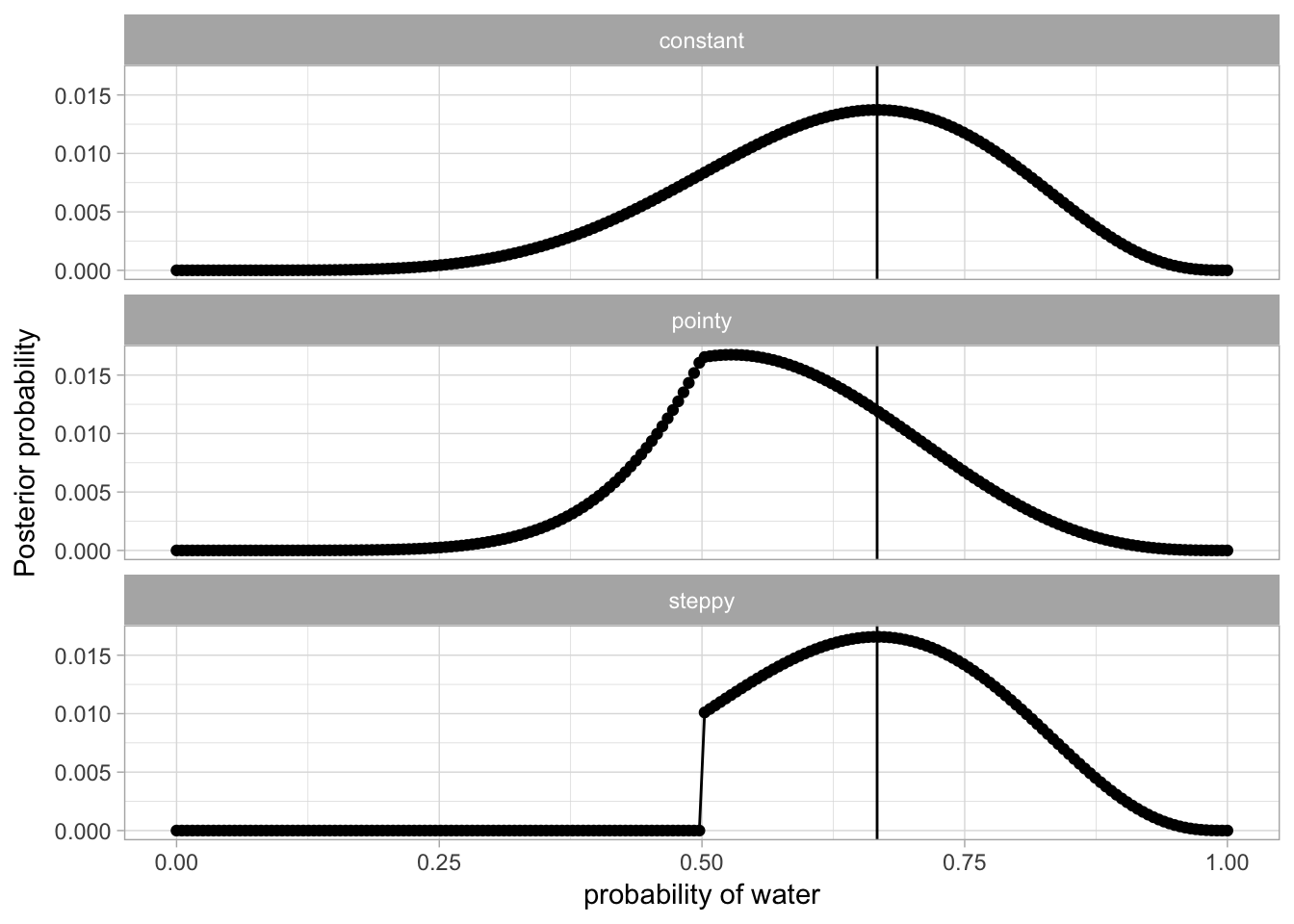

Interesting that the height of the curves varies – er, does that even mean anything? I guess it would impact the size of the HDPI, since more probability “mass” (I think that is the term) is piled up in a different place.

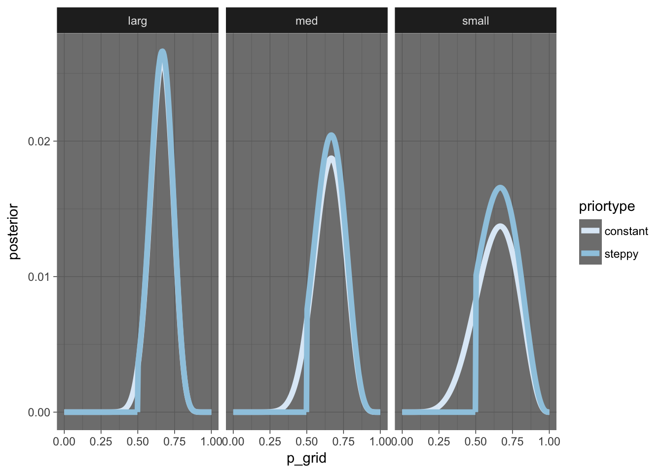
Curious that the step function seems to do the best! It says very little – just basically “at least half of the earth is water”. Though now that I think about it, it makes sense that the peak is higher – since the area below the curve is 1, more mass must have to get “shoved” under the peak here.

The pointy prior leads to pretty crappy results. I guess that makes sense, since it was a very confident, narrow prior that was totally wrong – the real value is not on 50% at all.

2.2 quadratic approx.

2.2.1 quick check to confirm it works

just a note. the text says

the logarithim of a gaussian distribution forms a parabola

I mean I could (will probably) check the math but can we just see?

curve(log(dnorm(x, 0, 1)), xlim = c(-2, 2))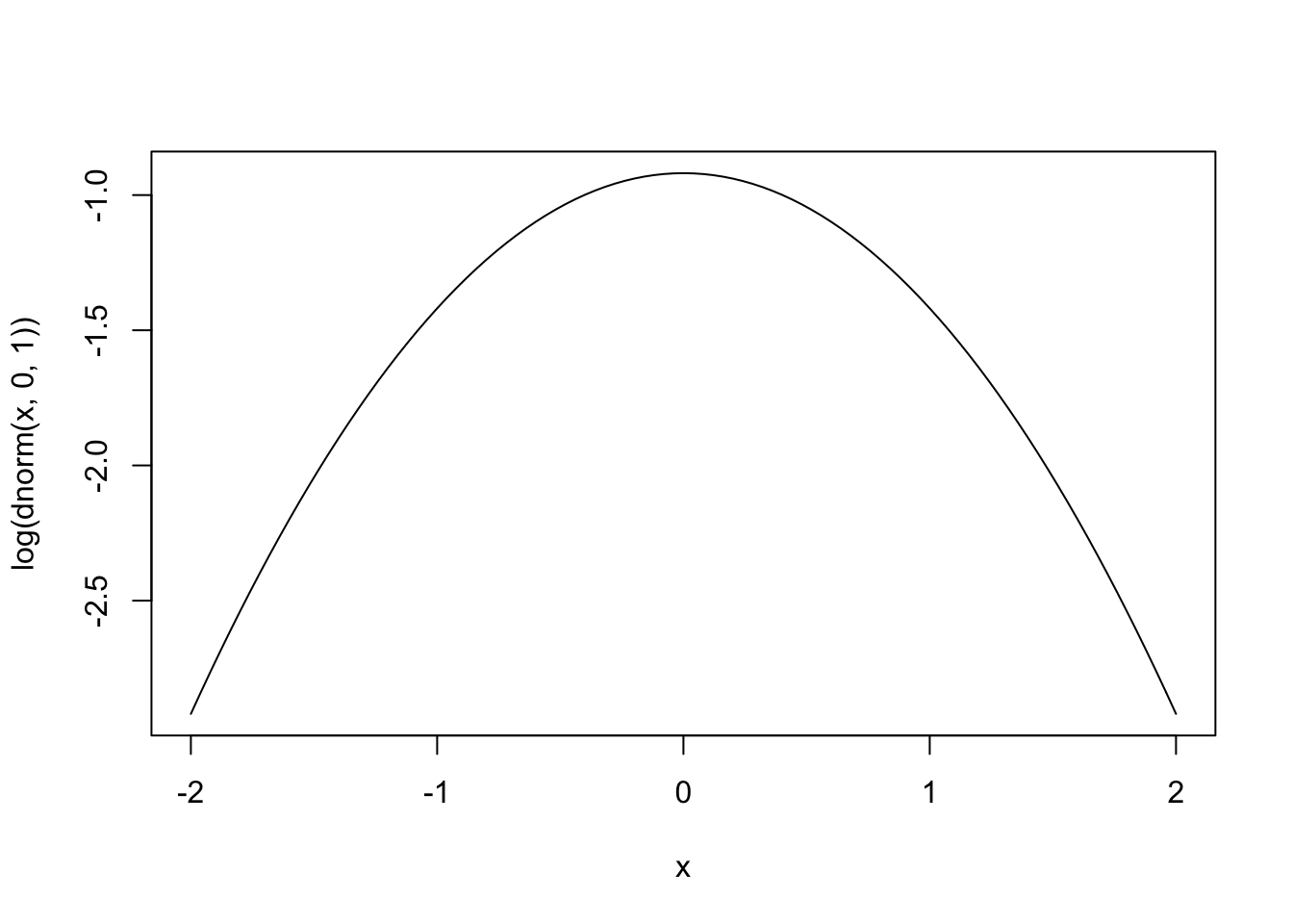

well i’ll be.

2.2.2 example from the text

Unfortunately, rethinking competes with map for the name of the function map().

globe.qa <- rethinking::map(
  alist(
    w ~ dbinom(9, p),         # I guess we know that we are always talking about 9 trials here? what if that was changing?
    p ~ dunif(0, 1)
  ), 
  data = list(w = 6)
)

str(globe.qa)

## Formal class 'map' [package "rethinking"] with 10 slots
##   ..@ call          : language rethinking::map(flist = alist(w ~ dbinom(9, p), p ~ dunif(0, 1)),      data = list(w = 6))
##   ..@ coef          : Named num 0.667
##   .. ..- attr(*, "names")= chr "p"
##   ..@ vcov          : num [1, 1] 0.0247
##   .. ..- attr(*, "dimnames")=List of 2
##   .. .. ..$ : chr "p"
##   .. .. ..$ : chr "p"
##   ..@ optim         :List of 7
##   .. ..$ par        : Named num 0.667
##   .. .. ..- attr(*, "names")= chr "p"
##   .. ..$ value      : num 1.3
##   .. ..$ counts     : Named int [1:2] 13 6
##   .. .. ..- attr(*, "names")= chr [1:2] "function" "gradient"
##   .. ..$ convergence: int 0
##   .. ..$ message    : NULL
##   .. ..$ hessian    : num [1, 1] 40.5
##   .. .. ..- attr(*, "dimnames")=List of 2
##   .. .. .. ..$ : chr "p"
##   .. .. .. ..$ : chr "p"
##   .. ..$ minuslogl  : num 1.3
##   ..@ data          :List of 1
##   .. ..$ w: num 6
##   ..@ start         :List of 1
##   .. ..$ p: num 0.583
##   ..@ formula       :List of 2
##   .. ..$ : language w ~ dbinom(9, p)
##   .. ..$ : language p ~ dunif(0, 1)
##   ..@ formula_parsed:List of 2
##   .. ..$ : chr "dbinom(x=w , 9 , p , log=TRUE)"
##   .. ..$ : chr "dunif(x=p , 0 , 1 , log=TRUE)"
##   ..@ fminuslogl    :function (pars)  
##   ..@ links         : list()

oy it is an S4 class!

globe_precis <- rethinking::precis(globe.qa)
rethinking:::precis_plot(rethinking::precis(globe.qa))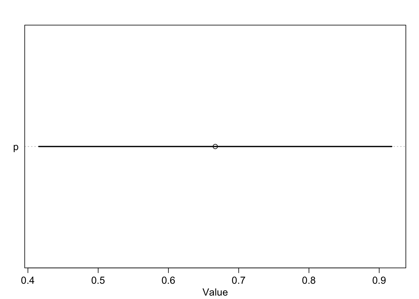

whoa it is all S4 classes! Calls for a bit of finesse to turn this into an attractive table:

globe.qa %>% 
  rethinking::precis(.) %>% 
  attr("output") %>% 
  mutate_all(round, digits = 2) %>% 
  knitr::kable()

Mean	StdDev	5.5%	94.5%
0.67	0.16	0.42	0.92

sample_sizes <- frame_data(~sample_size, ~samp,
           "small", c(6, 9),
           "med", c(12, 18),
           "larg", c(24, 36))


make_qa <- function(x){
  
  globe_qa <- rethinking::map(
    alist(
      w ~ dbinom(nt, p),         # I guess we know that we are always talking about 9 trials here? what if that was changing?
      p ~ dunif(0, 1)
    ), 
    data = list(w = x[1], nt = x[2])
  )
  
  out <- globe_qa %>% 
    rethinking::precis(.) %>% 
    attr("output")
  return(out)
}

QA_curve <- sample_sizes$samp %>% 
  purrr::map(make_qa) %>% 
  purrr::map(~ partial(dnorm, mean = .$Mean, sd = .$StdDev, .lazy = FALSE))

xs <- seq(0, 1, length.out = 200)
QA_curve %>% 
  invoke_map(list(list(x = xs))) %>% 
  purrr::map(~ data_frame(xs = xs, pred = .)) %>% 
  bind_rows(.id = "samplesize") %>% 
  ggplot(aes(x = xs, y = pred)) + 
  geom_line() + 
  facet_wrap(~samplesize)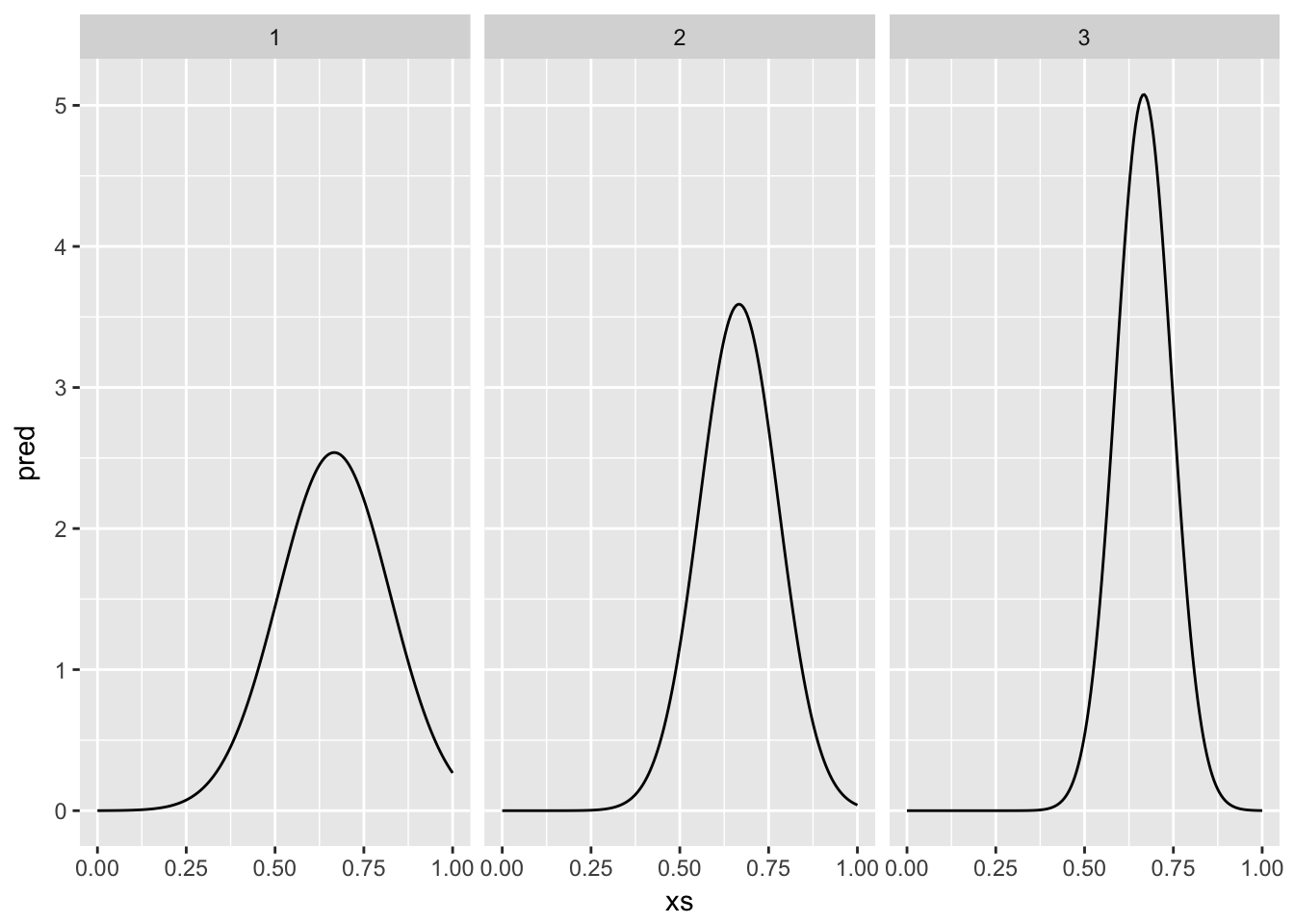

2.3 Practice

2.3.1 2E1

\(Pr(rain|Monday)\)

2.3.2 2E2

3 (probability that it is raining given that its monday)

2.3.3 2E3

1. \(Pr(Monday|rain)\)

2.3.4 2E4

Here goes. Probability describes the interaction of some kind of sampling process with something in the world. The surface of a globe is covered in some places with water, some with land - that’s fixed for any globe. When you toss a globe up in the air, the “probability of water” touching your finger when you catch it just describes the way you sample from that globe. You’ve turned the globe (which was just a globe) into a kind of weighted random number generator.

2.3.5 2M1

make_grid_approx <- function(f, s){
  data_frame(p_grid          = seq(from = 0, to = 1, length.out = 200),
             prior           = f(p_grid),
             likelihood      = dbinom(s[1], size = s[2], prob = p_grid),
             unstd.posterior = likelihood * prior,
             posterior       = unstd.posterior / sum(unstd.posterior))
}


sample_sizes <- frame_data(~sample_size, ~samp,
           "small", c(6, 9),
           "med", c(12, 18),
           "larg", c(24, 36))

prior_fns <- frame_data(~priortype, ~f,
                        "constant", function(x) 1,
                        "steppy", function(x) ifelse(x < 0.5, 0, 1))

setup_params <- tidyr::crossing(prior_fns, sample_sizes)

setup_params %>% 
  mutate(grid_approx = map2(f, samp, ~make_grid_approx(f = .x, s = .y))) %>% 
  tidyr::unnest(grid_approx) %>% 
  ggplot(aes(x = p_grid, y = posterior, colour = priortype)) + geom_line(size = 2) + facet_wrap(~sample_size) + scale_color_brewer() + theme_dark()