Chapter 3 Sampling the Imaginary
knitr::opts_chunk$set(echo = TRUE, cache = TRUE)
library(dplyr)
##
## Attaching package: 'dplyr'## The following objects are masked from 'package:stats':
##
## filter, lag## The following objects are masked from 'package:base':
##
## intersect, setdiff, setequal, unionlibrary(ggplot2)
library(purrr)3.1 Figures and text
grid_of_globe_toss <- data_frame(
  p_grid = seq(from = 0, to = 1, length.out = 1000),
  prior  = 1,
  likelihood = dbinom(6, size = 9, prob = p_grid),
  posterior_unstand = likelihood * prior,
  posterior = posterior_unstand / sum(posterior_unstand)
)

samples <- with(grid_of_globe_toss,
     sample(p_grid, prob = posterior, size = 1e4, replace = TRUE)
)

samples %>%
  data_frame(resampled = .) %>%
  ggplot(aes(x = resampled)) + geom_density()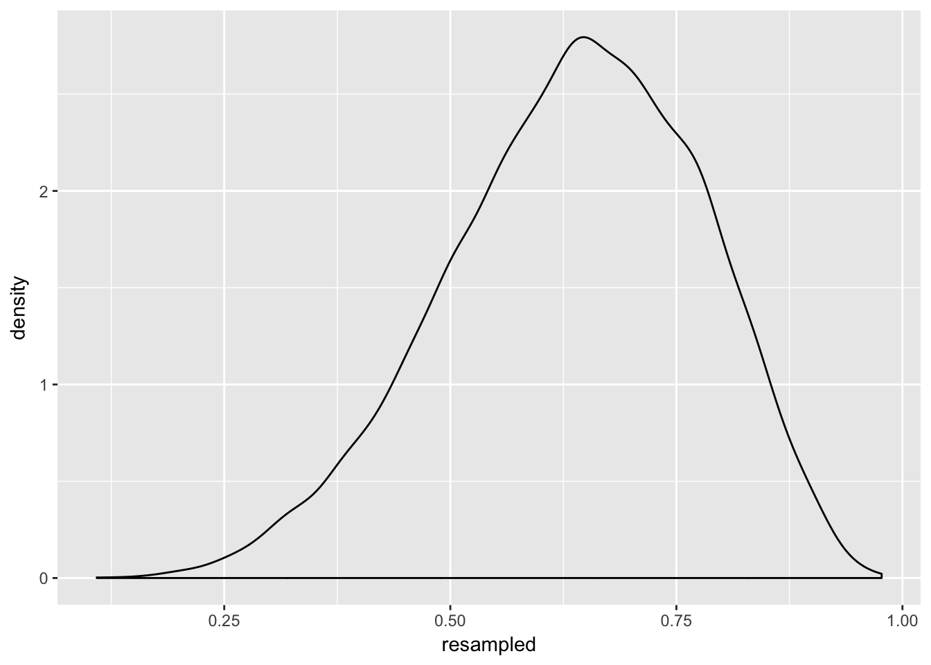
Here we have taken a very simple grid (that is, a simple list of 1000 numbers) and resampled it into 10 000 numbers (10x more). This is not necessary. but it does illustrate the point: you can use samples from the posterior to estimate its shape, and it works just as well as using the real thing.
sum(grid_of_globe_toss$posterior)## [1] 1with(grid_of_globe_toss, sum(posterior[ p_grid < 0.5 ]))## [1] 0.1718746its that last bit that we normally can’t do – picking out the values of p_grid. That’s because for other bigger models it is so complex we can’t answer that question accurately.
sum(samples < 0.5) / length(samples)## [1] 0.1729lo and behold, the value is nearly the same.
intervals <- list(
  c(-Inf, 0.5),
  c(0.5, 0.7)
)

sample_dens <- samples %>%
  density() %>%
  broom::tidy(.)

interval_density <- intervals %>%
  map(~ sample_dens$x > .x[1] & sample_dens$x < .x[2]) %>%
  map(~ sample_dens[.x,])

sample_dens %>%
  ggplot(aes(x = x, y = y)) + geom_line() +
  geom_polygon(data = rbind(interval_density[[1]], c(0.5, 0)))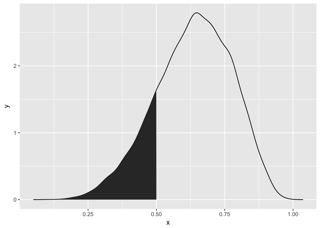
rethinking::HPDI(samples = samples, prob = 0.8)## |0.8 0.8|
## 0.4704705 0.82982983.2 simulation for prediction
rbinom(1e5, size = 9, prob = 0.7) %>%
  data_frame(dummy = .) %>%
  ggplot(aes(x = dummy)) +
  geom_histogram() +
  scale_x_continuous(breaks = 1:9)
## `stat_bin()` using `bins = 30`. Pick better value with `binwidth`.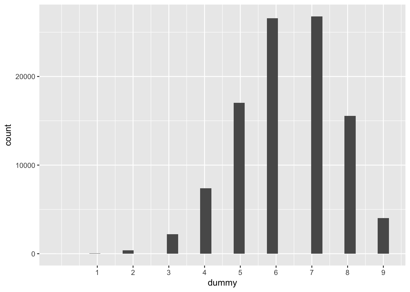
That shows you the expected distributions for one probability – 0.7. We need them at all such probablities
predicted_samples <- rbinom(length(samples), 9, prob = samples)

predicted_samples %>%
  data_frame(dummy = .) %>%
  ggplot(aes(x = dummy)) +
  geom_histogram() +
  scale_x_continuous(breaks = 1:9)
## `stat_bin()` using `bins = 30`. Pick better value with `binwidth`.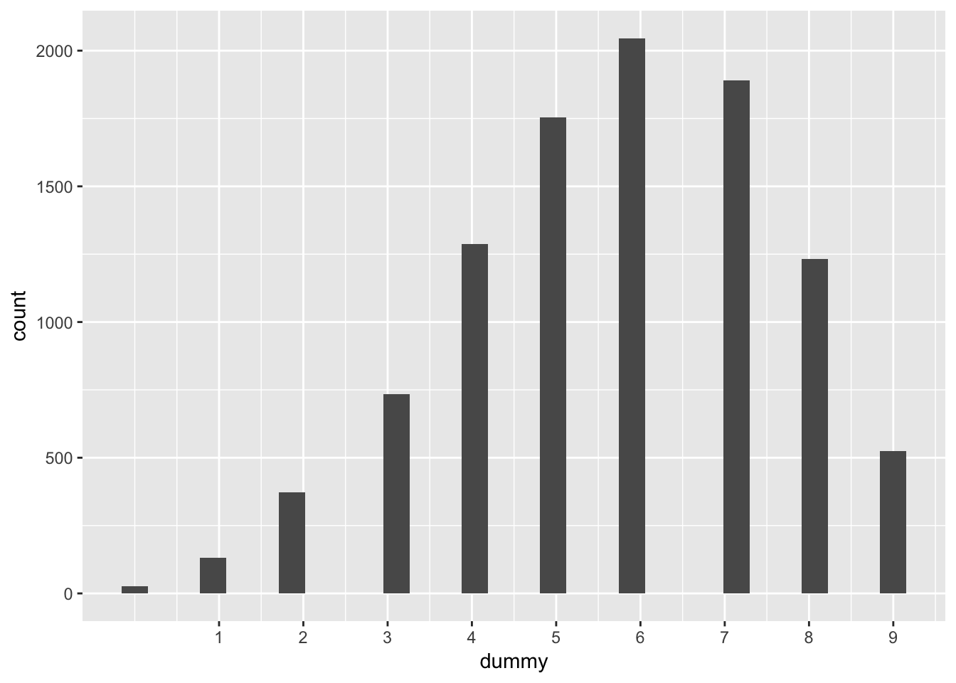
3.3 making breaking predicitons
repeated_single_samples <- map(samples, rbinom, n = 9, size = 1)

# should be able to get the histogram back
repeated_single_samples %>%
  map_dbl(sum) %>%
  data_frame(dummy = .) %>%
  ggplot(aes(x = dummy)) +
  geom_histogram() +
  scale_x_continuous(breaks = 1:9)
## `stat_bin()` using `bins = 30`. Pick better value with `binwidth`.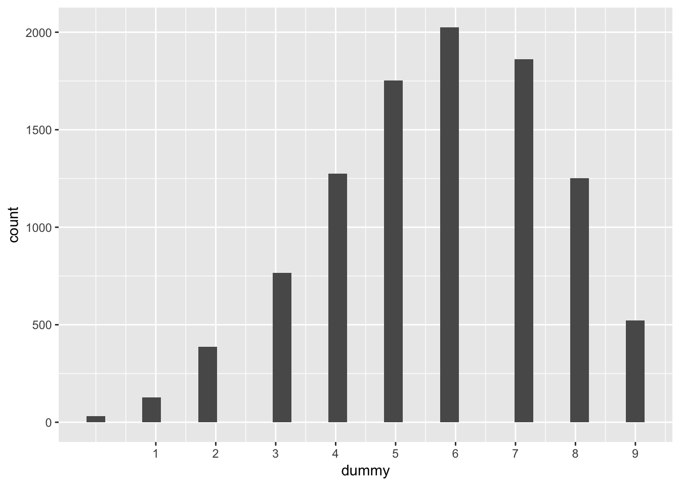
## can also calculate statistics about the temporal sequenc,e which is absent
## from the model

repeated_single <- repeated_single_samples %>%
  map(rle) %>%
  map_df(~ data_frame(n_switches = max(.x$lengths),
                      max_run    = length(.x$values)))

repeated_single %>%
  tidyr::gather(measure, value) %>%
  ggplot(aes(x = value)) +
  geom_histogram() + facet_grid(~measure)
## `stat_bin()` using `bins = 30`. Pick better value with `binwidth`.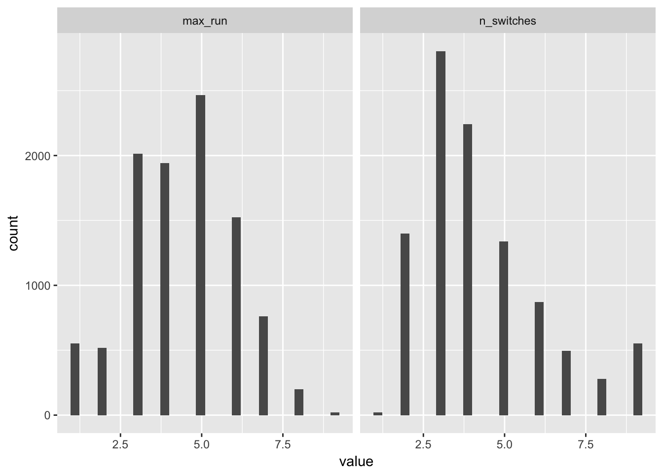
3.4 exercises
set.seed(100)
samples_exercise <- with(grid_of_globe_toss,
     sample(p_grid, prob = posterior, size = 1e4, replace = TRUE)
)
3.4.1 how much lies below p = 0.2 ?
below <- sum(samples_exercise < 0.2) / length(samples_exercise)about 0.05% below 0.2
3.4.2 how much lies above 0.8?
abv <- sum(samples_exercise > 0.8) / length(samples_exercise)11.17%
3.4.3 how much between 0.2 and 0.8
sum(samples_exercise < 0.8 & samples_exercise> 0.2) / length(samples_exercise)## [1] 0.88783.4.4 20% is below which value?
quantile(samples_exercise, 0.2)## 20%
## 0.51951953.4.5 20% is above which value?
quantile(samples_exercise, 0.8)## 80%
## 0.75675683.4.6 Which values contain the narrowest interval with 66% of posterior?
rethinking::HPDI(samples, 0.66)## |0.66 0.66|
## 0.5225225 0.7927928## just out of curiosity
plot(ecdf(samples))
abline(v = c(0.52, 0.8))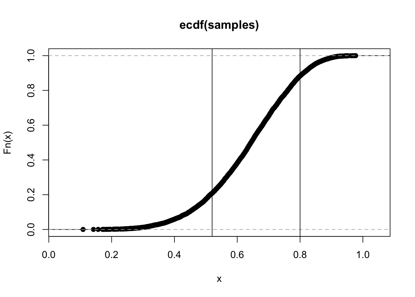
3.4.7 which values contain 66% of the variation, with equal amounts in the tails?
quantile(samples, c(0.16, 0.84))## 16% 84%
## 0.4924925 0.77877883.4.8 Medium
grid_of_globe_toss_15 <- data_frame(
  p_grid     = seq(from = 0, to = 1, length.out = 1000)      %>% rep(2),
  prior      = c(rep(1, 1000), rep(c(0,1), each = 500)),
  prior_is   = c("flat", "informative")                     %>% rep(each = 1000),
  likelihood = dbinom(8, size = 15, prob = p_grid),
  like_x_pri = likelihood * prior,
  posterior  = like_x_pri / sum(like_x_pri)
)

grid_of_globe_toss_15 %>%
  ggplot(aes(x = seq_along(posterior), y = posterior)) +
  geom_line() +
  facet_wrap(~prior_is, scales = "free")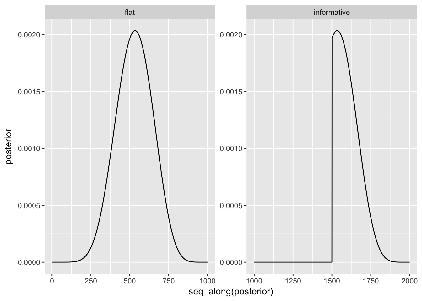
## sample from the posterior
posterior_samples <- grid_of_globe_toss_15 %>%
  split(., .$prior_is) %>%
  map(~ sample(.x$p_grid, size = 1e4,
               prob = .x$posterior, replace = TRUE)
  )

posterior_samples %>% map(rethinking::HPDI)
## $flat
## |0.89 0.89|
## 0.3373373 0.7207207
##
## $informative
## |0.89 0.89|
## 0.5005005 0.70770773.4.9 posterior predictive check
posterior_samples %>%
  map(~ rbinom(length(.x), size = 15, prob = .x)) %>%
  map_df(~ data_frame(posterior_pred = .), .id = "prior_is") %>%
  ggplot(aes(x = posterior_pred)) +
  geom_histogram(binwidth = 1) +
  geom_vline(xintercept = 8)+
  facet_grid(~ prior_is)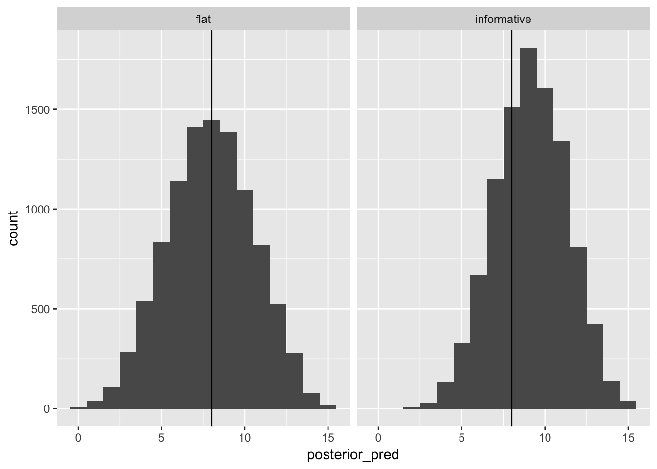
3.4.10 what is the probility of 6/9?
posterior_samples %>%
  map(~ rbinom(length(.x), size = 8, prob = .x)) %>%
  map(~ sum(.x == 6) / length(.x))
## $flat
## [1] 0.1506
##
## $informative
## [1] 0.20483.5 Hard
load in the data
library(rethinking)
homeworkch3 <- data(homeworkch3)
detach("package:rethinking", unload=TRUE)
library(purrr)
.. this does not work? all I get is the word “homeworkch3” which.. why would that even be.
Instead I will copy and paste the code for this example straight from Github
birth1 <- c(1,0,0,0,1,1,0,1,0,1,0,0,1,1,0,1,1,0,0,0,1,0,0,0,1,0,
0,0,0,1,1,1,0,1,0,1,1,1,0,1,0,1,1,0,1,0,0,1,1,0,1,0,0,0,0,0,0,0,
1,1,0,1,0,0,1,0,0,0,1,0,0,1,1,1,1,0,1,0,1,1,1,1,1,0,0,1,0,1,1,0,
1,0,1,1,1,0,1,1,1,1)
birth2 <- c(0,1,0,1,0,1,1,1,0,0,1,1,1,1,1,0,0,1,1,1,0,0,1,1,1,0,
1,1,1,0,1,1,1,0,1,0,0,1,1,1,1,0,0,1,0,1,1,1,1,1,1,1,1,1,1,1,1,1,
1,1,1,0,1,1,0,1,1,0,1,1,1,0,0,0,0,0,0,1,0,0,0,1,1,0,0,1,0,0,1,1,
0,0,0,1,1,1,0,0,0,0)
Test it to make sure that it works the same as the text:
sum(birth1) + sum(birth2)## [1] 111ok.
3.5.1 use grid approximation to estimate the posterior distribution of the probility of a male
male_babies <- data_frame(
  p_grid     = seq(from = 0, to = 1, length.out = 1000),
  prior      = 1,
  likelihood = dbinom(x    = sum(birth1) + sum(birth2),
                      size = length(birth1) + length(birth2),
                      prob = p_grid),
  like_x_pri = likelihood * prior,
  posterior  = like_x_pri / sum(like_x_pri)
)

male_babies %>%
  ggplot(aes(x = p_grid, y = posterior)) + geom_point()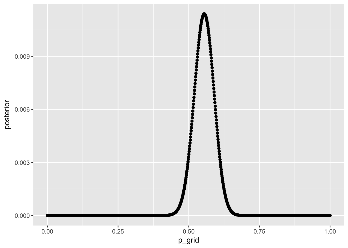
3.5.2 sample from the posterior distribution and get HPDI
male_babies_samples <- with(male_babies,
     sample(p_grid, size = 1e4, replace = TRUE, prob = posterior))

list(0.5, 0.89, 0.97) %>%
  map(rethinking::HPDI, sample=male_babies_samples)
## [[1]]
## |0.5 0.5|
## 0.5255255 0.5725726
##
## [[2]]
## |0.89 0.89|
## 0.5015015 0.6116116
##
## [[3]]
## |0.97 0.97|
## 0.4764765 0.62862863.5.3 simulate predictions
data_frame(sim_babies = rbinom(n = 1e4,
                               size = 200,
                               prob = male_babies_samples)) %>%
  ggplot(aes(x = sim_babies)) + geom_histogram(binwidth = 1) +
  geom_vline(xintercept = 111)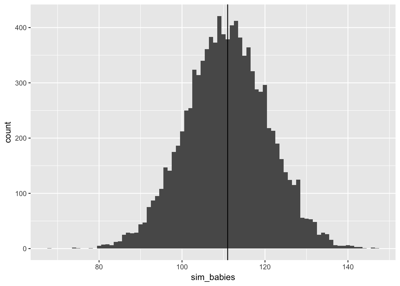
3.5.4 now, using the same posterior for all births, consider the first born only!
data_frame(sim_babies = rbinom(n = 1e4,
                               size = length(birth1), #100
                               prob = male_babies_samples)) %>%
  ggplot(aes(x = sim_babies)) + geom_histogram(binwidth = 1) +
  geom_vline(xintercept = sum(birth1))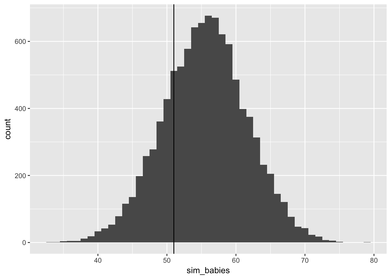
the model overestimates firstborn? I wonder if these data are from a society that really values boys? Such that if you have a daughter first then you try again, hoping for a boy. But if you start with a boy then you stop, and you wouldn’t be in this sample (which is two-child families only)
3.5.5 simulate boys after girls
If I was right above, the model should underestimate these births!
Ok so first we need to know where the girl babies are in the first vector
## how many births after girls?
length(birth2[birth1 == 0])
## [1] 49## how many of those were boys?
sum(birth2[birth1 == 0])## [1] 39data_frame(sim_babies = rbinom(n = 1e4,
size = 49, #total births after girls
prob = male_babies_samples)) %>%
ggplot(aes(x = sim_babies)) + geom_histogram(binwidth = 1) +
geom_vline(xintercept = sum(birth2[birth1 == 0]))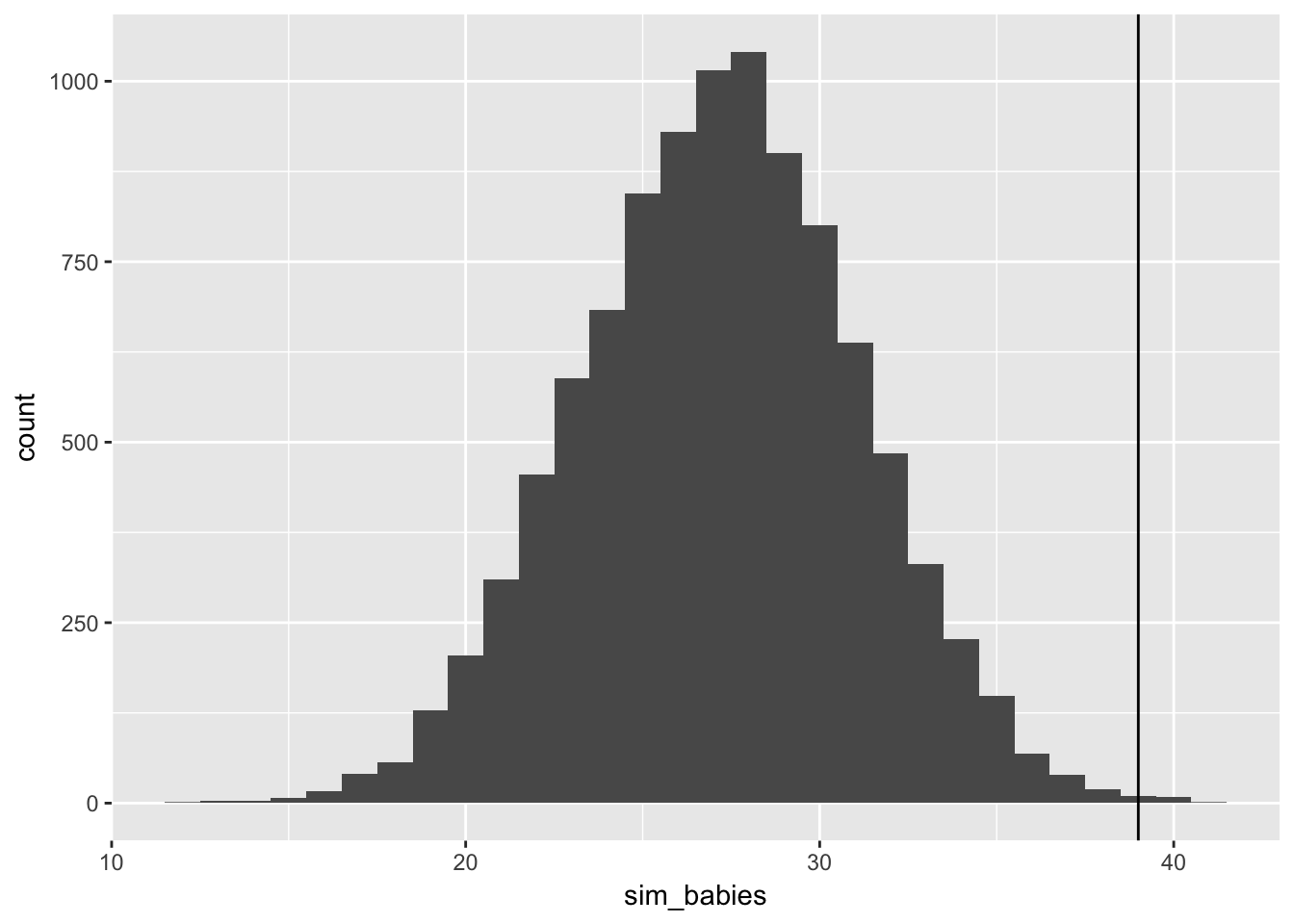
Wow, it definitely does underestimate it! it does a terrible job of guessing at the sex of a second birth.